Simulation-based prediction of the thermal process emission measured by pyrometry of 316L stainless steel

Laser powder bed fusion is a common additive manufacturing process in which metal powder is selectively melted by a laser. Meandering stripe hatching is often used in conjunction with constant process parameters such as laser power and scan speed. However, the exposure strategy and the part geometry influence the resulting melt pool. To compensate for these influences, closed-loop process control based on the thermal emission can be used. To enable closed-loop process control via pyrometry, an analysis of the measured thermal emissions is necessary, as the measurement spot of the pyrometry is larger than the melt pool.

This article investigates how accurately the pyrometrically measured thermal emission can be predicted by a thermal simulation and how large the influence of the neighboring vectors is on the pyrometrically measured thermal emission. For this purpose, a thermal simulation model is first developed that considers the immediate environment (approx. 1 mm) of a single scan vector. Subsequently, a model is developed that predicts the thermal emission within the measuring spot of the pyrometer based on the simulated temperature. The results show the thermal emission prediction model provides an accurate prediction with an average deviation of approx. 4.5%. The evaluation of the influence of neighboring vectors also shows that in areas of small vectors, the pyrometrically measured thermal emission is caused by neighboring vectors by approx. 35%. In further investigations, the influence of the neighboring vectors in the setpoint of the controller is to be considered.

1 Introduction

For the production of L-PBF parts, meandering stripe hatching is often used in conjunction with constant process parameters such as laser power and scan speed [1-2]. The melt pool is influenced by the interaction of the energy input determined by the process parameters, the preheating, e.g. by the exposure strategy, and the part related heat dissipation, i.e. the part geometry [1, 3-7]. This leads to a geometry-dependent part quality. For example, [8] demonstrates a local elevation of 22 µm at turning points when using a meander exposure strategy. The local elevation is caused by the preheating of the previously exposed vectors. To compensate for these influences, closed-loop process control based on the thermal emission can be used.

Thermal emission refers to the heat radiation generated during the process, which is detected using pyrometry. Closed-loop process control offers a cost-effective and simple approach to automated parameter adaptation [9]. The AconityCONTROL (Aconity3D GmbH, Germany, Herzogenrath) control system compares the measured thermal emission with a constant reference value and regulates the resulting thermal emission via the laser beam power. The controller updates the control variable (laser power) at intervals of 10 µs [10]. The speed of the update in conjunction with the assumption that the pyrometrically measured signal can be used to evaluate the melt pool temperature makes closed-loop control appear promising, particularly with regard to increasing process robustness [10]. The investigations on several tracks show the preheating caused by the exposure strategy in particular can be measured via an on-axis pyrometer [9, 11].

The investigations of the thermal emission during the exposure of single vectors show the thermal emission allows conclusions to be drawn about the aspect ratio of the keyhole. A linear-proportional relationship can be demonstrated between the thermal emission normalized to the square of the beam diameter and the aspect ratio of the keyhole [12]. Investigations by Kavas et al. [10] show the use of a constant controller setpoint nonetheless leads to pore formation, especially in the case of small vector lengths. The spot size of the pyrometer in the L-PBF process is usually larger than the melt pool. The measuring spot size depends on the optical setup and therefore varies in the previous investigations. In most cases, however, the measuring spot is large enough to detect at least one neighboring melt track that has already been exposed. The neighboring melt tracks that have already been exposed are referred to as neighboring vectors.

One possible cause for the formation of pores when using process control is the thermal emission generated by neighboring vectors. In this publication, the influence of neighboring vectors is simulatively investigated in order to identify this as a source of error. Two models are developed for this purpose: The first model simulates the temperature field generated during the process. The second model is then used to predict the thermal emission, which is measured using pyrometry. Numerous studies have already presented simulation models for the L-PBF process [13]. However, there is currently a lack of models that predict or examine in more detail the thermal emission measured using pyrometry. The methodology section first describes the manufacturing process used to evaluate the simulation and calculate the emissivity. The two models are presented in the following sections. The results of the investigation are described and discussed in Section 5.

2 Methodology

Two models will be developed that enable the prediction of thermal emission. To evaluate the accuracy of the prediction and to calculate the emissivity, test specimens are built and the resulting thermal emission is measured via an on-axis pyrometer. The specimens are cylindrical with triangles in the center (see Figure 1), resulting in areas with small vector lengths.

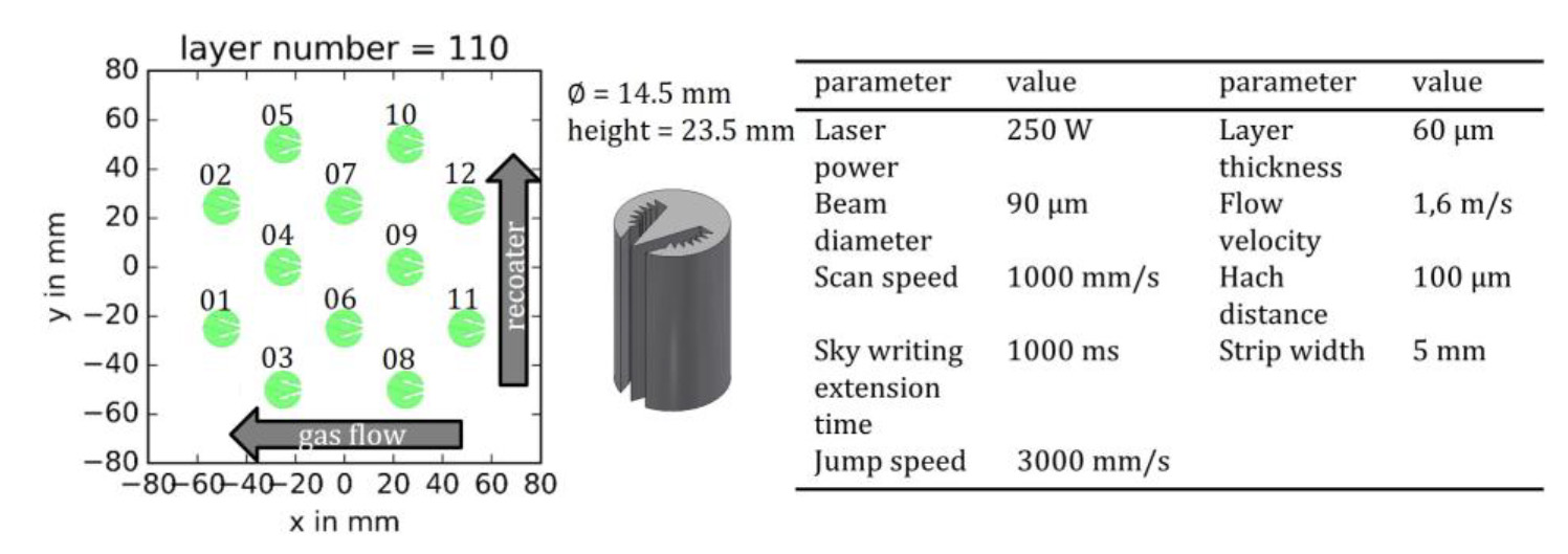
The samples are manufactured on an L-PBF machine AconityMIDI (Aconity3D GmbH, Germany, Herzogenrath). The AconityMIDI is equipped with a 1,200W AFX-1000 laser (nLIGHT, United States, Washington). The samples are made from 1.4404 powder “m4p™ 316l” (m4p material solutions GmbH, Austria, Feistritz i. R.) with an average grain size of 45 µm. The thermal radiation generated in the process is detected in the wavelength range from 2.0 µm to 2.2 µm with a measuring frequency of 100 kHz using a customized non-linearized KG 740-LO pyrometer (Kleiber Infrared GmbH, Unterwellenborn, Germany). Due to the lack of linearization, the emissivity set on the pyrometer corresponds to a division of the measurement signal by the emissivity. To maximize the measurement signal, the emissivity is set to 0.1, which corresponds to the minimum adjustable emissivity.

The build platform is preheated to a temperature of 100°C to produce the test specimens. The process parameters used for production are listed in Figure 1. The samples are exposed in sequence (part 1 to 12) against the inert gas flow in order to reduce the influence of spatter. A meandering stripe hatching is used as the exposure strategy, which is rotated by 33° layer by layer. Vector directions with an angle of less than 45° to the shielding gas flow are omitted in order to reduce the interaction of the laser beam with the metal vapor, cf. [14].

3 Thermal simulation model

For the thermal simulation, a model is developed that only considers the environment of an exposure vector. This approach makes it possible to map pre-heating effects due to the exposure strategy while keeping the numerical effort to a minimum. The model is programmed in Python and is based on the finite difference method.

Figure 2a shows an example of the calculation area for different vectors. The simulated scan vector is shown in red. The size of the calculation area depends on the length of the exposure vector. The origin of the calculation area is always at the starting point of the exposure vector, while the exposure direction is the X-axis of the calculation area. This means the calculation area rotates relative to the part depending on the orientation of the exposure vector. The advantage of the described calculation area is that the meshing only has to be carried out once, as the meshed grid is only shifted or rotated. A structured grid with different element sizes in the Z-direction is used for meshing.

Figure 2a shows that, in the area of the laser-material interaction, the mesh is finest in the Z-direction (element height = layer thickness). From a given number (n₁) of elements, the element size in the Z-direction is doubled. The number of elements in the Z-direction is n_z = 12. The element size is doubled after n₁ = 6. The element size in the X- or Y-direction corresponds to the track spacing (100 µm). This corresponds to the largest possible element size for mapping the exposure vectors. The number of elements in the Y-direction is n_y = 21, and the number of elements in the X-direction is determined by the length of the longest exposure vector of a layer to be simulated and a specified edge distance of seven elements.

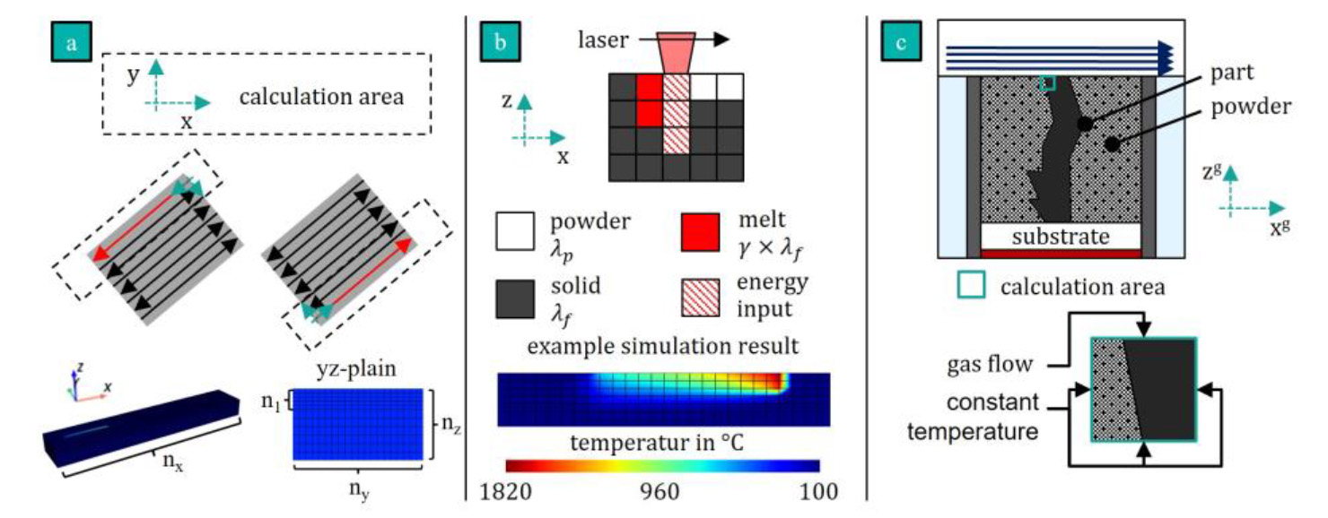
The part layers of the part to be simulated are simulated independently of each other, i.e. preheating by already exposed layers is neglected. To simulate a layer, the vector information is loaded from a CLI (common layer interface) file. The element state (powder or solid) is also assigned based on the CLI file. When starting the simulation of a layer, the temperature of all elements is set to the preheating temperature (see Section 2). As a boundary condition, it is assumed that the global part temperature corresponds to the preheating temperature, so that the side surfaces and the bottom surface of the calculation area are set to the preheating temperature as a constant boundary condition (see Figure 2c).

The upper surface of the calculation area borders on the shielding gas flow. In order to map the shielding gas flow in the simulation, the mean heat-transfer coefficient with forced convection is calculated for a longitudinally flowing flat plate with laminar boundary layer according to [15]. It is assumed the shield gas has a temperature of 60°C, and the characteristic length l is equal to the diameter of the substrate plate (170 mm).

The calculation of the material values is based on references [15-21]. Due to the melt pool dynamics, which cannot be represented by the purely thermal simulation, more heat is dissipated from the melt pool (cf. [22]). In order to take the influence of Marangoni convection into account in the thermal simulation, the thermal conductivity within the melt can be artificially increased by a correction factor γ = 3 [23] (cf. [8]). In the simulation model, the enthalpy of melting is neglected for the purpose of simplifying the model. However, this can be incorporated into the specific heat capacity in subsequent investigations. The thermal conductivity of the powder λ_p is calculated according to the equation by Meredith and Tobias [24]. To calculate the thermal conductivity of the powder, the volume ratio ϕ of solid to gas is estimated at 70%.

The specific heat capacity c_g and the density ρ of the powder are calculated from the volume ratio of the solid and gas properties. To map the energy input by the laser, a cuboid volume with a constant heat flow is used as the heat source, cf. [25]. The power density W is calculated according to W = P_lμ_l/ℎ²Δz_sn_w with the laser power P_l, the absorption coefficient μ_l, the track spacing h, the layer thickness Δz_s and the number of elements n_w. The number of elements nw represents the depth of the melt pool in the Z-direction. The energy input takes place in nw elements in the Z-direction. Figure 2b shows the heat source for n_w = 3 and the simulated temperature of an exposure vector in a cutaway drawing. The elements where the energy input occurs are shaded. The absorption coefficient is assumed to be 60% and indicates the proportion of the laser power that is absorbed by the molten pool, cf. [25].

4 Prediction of thermal process emissions

To predict the thermal emission, the emission of the elements located in the measuring spot of the pyrometer is calculated. The size of the measuring spot is determined by scanning an aperture (diameter = 1 mm) with a radiation source underneath. The determined measuring spot of the pyrometer is 0.94 mm. The manufacturer of the pyrometer specifies the relationship between output value and temperature for linearization. Assuming that each element within the measurement spot is included in the measurement signal to the same extent, the output value is calculated in relation to the measurement spot area. This relationship is used to calculate an output value field from the simulated temperature field.

This output value field is then multiplied by the emissivity of the material and divided by the emissivity set on the pyrometer (see section 2). The sum of the output values gives the predicted signal of the pyrometer. Two emissivity values are used to predict the thermal emission, the first for temperatures below 1,000°C and the second for temperatures above 1,000°C. To determine the emissivities, both emissivities are varied in a range from 0 to 1 for the prediction of the emission of 15 layers and the deviation from the measured signal is determined. The combination of emissivities that results in the smallest deviation is used to predict the thermal emission. To calculate the deviation between the predicted and measured signal, the emission of all built-up samples is averaged and reduced to the resolution of the simulation. To reduce the resolution, the measured values within an element are averaged.

5 Results and discussion

The averaged measured thermal emission signal for an exemplary layer 110 is shown in Figure 3. The emissivities that lead to the smallest deviation between the predicted and measured signal are: ε_ϕ<=1,000°C = 0.482 and ε_ϕ>1000°C = 0.131. A comparison with values from the literature shows that, despite differing absolute values, the ratio is of a similar magnitude: ε_{ϕ=700°C, sandblasted} = 0.7 and ε_{ϕ>1600°C, ϕ<1800°C} = 0.28 [26]. The prediction of the thermal emission provides an accurate prediction with an average deviation of 4.5% (9.4 mV) for layers 100 to 150. The deviation is greatest at the edges of the stripes.

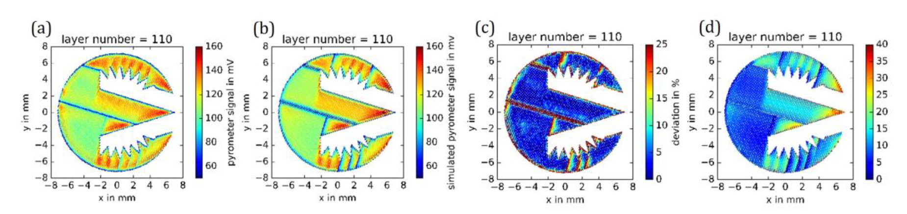
This deviation is probably due to the neglect of the pre-heating of already exposed strips. With each shift of the calculation area, the preheating temperature is assigned to the elements that lie outside the calculation area of the last time step. Particularly in the case of step vectors, this procedure means that local part overheating is no longer considered. Despite the existing deviation, the thermal simulation can map the preheating effects caused by the exposure strategy and enables a prediction of the thermal radiation generated in the process. Figure 3 shows the signal component caused by the thermal emission of neighboring vectors.

To calculate the proportion of neighboring vectors, the signal proportion of the area with a temperature below 1,000°C is evaluated in a simplified manner. The signal component increases to approx. 35%, especially in the area of small vectors. The influence of neighboring, not yet completely cooled vectors on the measured thermal emission is possibly the reason for the observation that the porosity increases when using a closed-loop process control.

6 Conclusion and future work

This publication presents a model for thermal simulation of the L-PBF process and a model for predicting the resulting thermal emission. With both models, the resulting process emission can be predicted with an average deviation of 4.5%. Since the simulation presented has only been experimentally validated for one material and one set of parameters, further investigations involving a comprehensive uncertainty study must be carried out. For example, it can be investigated whether the prediction of thermal emission is possible with similar accuracy when the laser power is varied. Furthermore, it is shown that a part of the pyrometrically measured thermal emission is caused by neighboring vectors.

However, this conclusion is based solely on a simulation study, which is why further investigations must be carried out to confirm this assumption. One possibility would be to investigate the melt pool geometry in the area of small vectors by micrographs and compare it with the measured increase in thermal radiation. However, predicting the thermal emission to define a variable controller setpoint seems promising. A variable controller setpoint could consider the thermal emission of neighboring vectors in advance. This would prevent excessive power reduction and enable closed-loop process control, which can lead to higher part quality. In addition, a direct adjustment of the laser power based on thermal simulation will be further investigated. As part of this investigation, a sensitivity analysis will be carried out to evaluate the influence of the assumptions made on the simulation result. It may be possible to achieve a significant reduction in part defects by using a hybrid simulation-based control concept. 

•This article (https://iopscience.iop.org/article/10.1088/1757-899X/1332/1/012033) is an open access article distributed under the terms and conditions of the Creative Commons Attribution (CC BY) license (https://creativecommons.org/licenses/by/4.0/). The article has been edited to conform to the style of Thermal Processing magazine.

References

1. Yeung H., Lane B. 2020 Manufacturing Letters 25 56-59.
2. Duong E., Masseling L., Knaak C., Dionne P., Megahed M. 2022 Additive Manufacturing 3 100047.
3. Criales L. E., Arısoy Y. M., Lane B., Moylan S., Donmez A., O zel T. 2017 International Journal of Machine Tools and Manufacture 121 22-36.
4. Phutela C., Aboulkhair N. T.; Tuck C. J., Ashcroft I. 2019 materials 13 117.
5. Langhorst M. 2015 Beherrschung von schweißverzug und schweißeigenspannungen dissertation Technischen universita t mu nchen.
6. Hooper, P. A. 2018 Additive Manufacturing 22 548-559.
7. Williams R. J., Piglione A., Rønneberg T., Jones C., Pham M., Davies C. M., Hooper P. A. 2019 Additive Manufacturing 30 100880.
8. Pichler, Tobias Adaptives laser powder bed fusion der titanlegierung TiAl6V4 dissertation rheinisch-westfa lischen technischen hochschule Aachen.
9. Hagedorn Y., Pastors F. 2018 Laser Technik Journal 15 54-57.
10. Kavas B., Balta E. C., Tucker M. R., Krishnadas R., Rupenyan A., Lygeros J., Bambach M. 2025 Additive Manufacturing 99 104641.
11. Renken V., Freyberg A., Schu nemann K., Pastors F., Fischer A. 2019 Progress in additive manufacturing 4 411-421.
12. Stajkovic J., Kahl M., Kaserer L., Braun J., Scheuringer S., Mayr-Schmo lzer B., Distl B., Leichtfried G. 2024 Journal of Manufacturing Processes 141 1310-1323.
13. Bayat M., Dong W., Thorborg J., To A. C., Hattel J. H. 2021 Additive Manufacturing 47 102278.
14. Schniedenharn M. 2020 On the influence of focal shift and process by-products on the laser powder bed fusion process dissertation rheinisch-westfa lischen technischen hochschule Aachen.
15. Stephan P., Kabelac S., Kind M., Mewes D., Schaber K., Wetzel T. 2019 VDI-Wärmeatlas Springer.
16. Ho C. Y., Powell R. W., Liley P. E. 1972 Journal of Physical and Chemical Reference Data 2 279-421.
17. MacBride B. J., Gordon S., Reno M. A. 1993 Thermodynamic data for fifty reference elements NASA.
18. Kestin J., Knierim K., Mason E. A., Najafi B., Ro S. T., Waldman M. 1984 Journal of Physical and Chemical Reference Data 13 229-303.
19. Kim C. S. 1975 thermophysical properties of stainless steels Argonne national laboratory.
20. Yamada N., Okaji M., Miki Y. 1995 The fourth asian thermophysical properties conf. last viewed on 1995 Tokyo.
21. Mills K. C. 2002 Recommended values of thermophysical properties for selected commercial alloys Woodhead.
22. Cox B., Ghayoor M., Doyle R. P., Pasebani S., Gess J. 2022 The international journal of advanced manufacturing technology 9-10 5715-5725.
23. Nikam S. H., Quinn J., McFadden S. 2021 Numerical Heat Transfer, Part A: Applications 79 537-552.
24. Meredith R. E., Tobias C. W. 1960 Journal of Applied Physics 31 1270-1273.
25. Keller N. 2016 Verzugsminimierung bei selektiven laserschmelzverfahren durch multi-skalen-simulation dissertation Universita t Bremen.
26. Emissionsgradtabelle last viewed on 07/06/2025 available online: www.kleiberinfrared.com/index.php/de/amanwendungen/emissionsgrade.html.