Quench factor analysis: C-curve determination

Previously, I discussed the concept of the quench factor, as developed by Staley [1]. We showed that it was possible to determine properties as a function of quench rate using the Jominy end quench. In this column, I will discuss the C-curve and the determination of the coefficients of the C-curve.

Introduction

The C-curve is like the Time-Temperature-Transformation curve for continuous cooling. In general, the C_t function is described as [1]:

where C_t is the critical time required to precipitate a constant amount of solute. The meaning of each of the constants are described in my previous article.

To determine the parameters K₁, K₂, K₃, K₄, and K₅, it is first necessary to have the C-curve. C-curve data is scarce and of limited availability. Some Time-Temperature-Property curves have been collected [2]. Some coefficients for the C_t function are shown in my previous column and in [3]. Once the C-curve, or Time-Temperature-Property curve, is obtained, the values of the coefficient are obtained by repeated iterations (and minimum error) until the best fit to the C-curve is achieved [4].

Determination of the C-curve

From the above discussion, the quench factor, τ, can be determined for any position on the Jominy end quench with hardness measurements. Since the quench factor is related to the C-curve by the relationship:

Or:

In the Jominy end quench, an infinite number of quench rates are available, and the path is known from the relationship described by [5]. It is important to understand that the cooling rates can change due to the changes in thermal conductivity of aluminum due to alloying content.

Based on this relationship, the time increments, ∆t₁, ∆t₁, ∆t₃, through ∆t_n, can be determined by examining the quench path, and dividing the critical temperature range (400°C through 200°C) into intervals at specific temperatures. Since the C-curve is independent of the quench path, a series of nonlinear equations can be established to solve for the critical time, C_t for different quench factors:

where τ₁, τ₂, τ₃. … τ_n are the quench factors from locations on the Jominy end quench specimen; ∆t₁, ∆t₁, ∆t₃, through ∆t_n are the temperature intervals from the quench path at specific locations on the Jominy end quench, and C₁, C₂…C_n are the critical times on the C-curve.

Solution of this set of equations will provide the C-curve, or critical time as a function of temperature. To minimize false and unrealistic answers, it is necessary to constrain the results of the solution to the series of nonlinear equations solved above. Examples of the constraints used are the stipulation that all solutions for C_t must be positive and not equal to zero. Further, the results are constrained to yield results C_t less than 5,000. Examination of the data available [4] [6] [7], indicates that this is a reasonable assumption. Better solutions for the shape of the C_t curve would be obtained with more nonlinear equations.

Gandikota [6] provides a program for the simultaneous solution to the above equations. Once the C-curve is obtained, calculation of the constants K₂, K₃, K₄, and K₅ is difficult, because of the very nonlinear nature of the equations. However, the use of thermodynamic data as suggested by Shuey and Tiryakioglu [7] [8] simplify analysis. Further improvement can be achieved by the implementation of the improved quench factor model of Rometsch [9] or Tiryakioglu [7] [8].

Problems with the equation for the C-curve are its complex nature and dependence on K₂–K₅. Different sets of K₂–K₅ can provide similar fits to the data, with similar errors, but can provide wildly different Time-Temperature-Property curves [7]. Fitting the Time-Temperature-Property coefficients is severely non-linear, and results in errors regardless of the method used. Independent physical data offer much better fits to the data and result in reduced errors in the C-curve. Data such as the solvus temperature (K₄), solute diffusivities (K₅), and enthalpy for precipitation (K₇) substantially reduce the fitting errors and non-linearity and offer physical meaning to the data and fit. Use of the thermodynamic data also drastically reduces the computational load. Use of many data points (> 10) reduces the errors. Combining interrupted quench data and continuous cooling data is very effective in reducing C-curve errors.

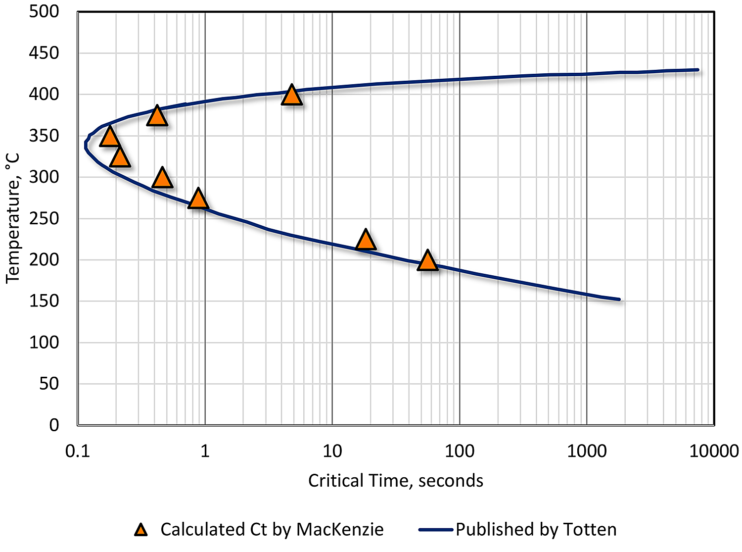
An example of such a solution is shown in Figure 1. The data fit published data well, within the constraints cited by others [9] [10] [7]. This data demonstrates the usefulness of the technique and is a powerful tool to be used for the prediction of properties resulting from changes in heat treatment.

Conclusions

In this column, we have described a method of determining the C-curve for aluminum, using the Jominy end quench. From the C-curve, we can calculate the coefficients in the C_t function, and then be able to calculate properties. Since properties are also a direct function of the quench rate, the quench factor can be directly determined from the Jominy end quench as a function of distance from the quenched end, or quench rate in the critical range of 400°C through 200°C.

Should you have any suggestions for additional columns, or have questions regarding any column, please contact the editor or myself. 

References

1. J. T. Staley, “Quench Factor Analysis of Aluminum Alloys,” Mat. Sci. Tech., vol. 3, p. 923, November 1987.
2. H. Chandler, Ed., Heat Treater’s Guide: Practices and Procedures for Nonferrous Alloys, Materials Park, OH: ASM International, 1996.
3. D. S. MacKenzie, “Metallurgy of Heat Treatable Aluminum Alloys,” in Heat Treating of Nonferrous Alloys, vol. 4E, G. E. Totten and D. S. MacKenzie, Eds., Materials Park, OH: ASM InternationAL, 2016, p. Metals Handbook 2A.
4. J. W. Evancho and J. T. Staley, “Kinetics of Precipitation in Aluminum Alloys During Continuous Cooling,” Met. Trans., vol. 5, pp. 43-47, January 1974.
5. G. P. Dolan, R. J. Flynn, D. A. Tanner and J. S. Robinson, “Quench factor analysis of aluminum alloys using the Jominy end quench technique,” J. Mat. Sci. Tech., vol. 21, no. 6, pp. 687-692, 2005.
6. V. Gandikota, “Quench Factor Analysis of Wrought and Cast Aluminum Alloys, PhD Dissertation,” 2009.
7. R. T. Shuey, M. Tiryakioglu and K. B. Lippert, “Mathematical Pitfalls in Modeling Quench Sensitivity of Aluminum Alloys,” in Proc. 1st Intl. Sym. Metallurgical Modeling for Aluminum Alloys, 13-15 Oct. 2003, Pittsburgh, PA, 2003.
8. M. Tiryakioglu and R. T. Shuey, “Multiple C-Curves for Modeling Quench Sensitivity of Aluminum Alloys,” in Proc. 1st Intl. Sym. Metallurgical Modeling for Aluminum Alloys: 13-15 October, 2003, 2003.
9. P. A. Rometsch, M. J. Starink and P. J. Gregson, “Improvements in Quench Factor Modeling,” Mat. Sci. Eng., vol. A339, pp. 255-264, 2003.
10. R. T. Shuey and M. Tiryakioglu, “Quenching of Aluminum Alloys,” in Quenching Theory and Technology, B. Liscic, H. Tensi, L. C. Canale and G. E. Totten, Eds., Boca Raton, FL: CRC Press, 2010, pp. 43-84.
11. D. S. MacKenzie, Quench Rate and Aging effects in Al-Zn-Mg-Cu Aluminum Alloys, PhD Dissertation, Rolla, MO: University of Missouri – Rolla, 2000.
12. G. E. Totten, G. M. Webster and C. E. Bates, “Quenching,” in Handbook of Aluminum: Volume 1 Physical Metallurgy and Processes, G. E. Totten and D. S. MacKenzie, Eds., Boca Raton, FL: Marcel Dekker, 2003, p. 975.
13. G. E. Totten, C. E. Bates and L. M. Jarvis, Heat Treating, p. 16, December 1991.