


Introduction
Recent developments have been made in the field of powder metallurgy of materials to obtain advanced properties as compared to conventional manufacturing of materials for various applications. Powder metallurgy offers several advantages like improved strength and dimensional stability resulting in near net-shape products. Development of powder metallurgy techniques has resulted in new primary and secondary fabrication routes for semi-finished products. Numerous consolidation methods have been implemented to produce components with superior microstructure and mechanical properties [1]. Properties and performance of these powder metallurgy components rely heavily on the type of manufacturing process selected. One such manufacturing process in powder metallurgy is solid-state sintering.
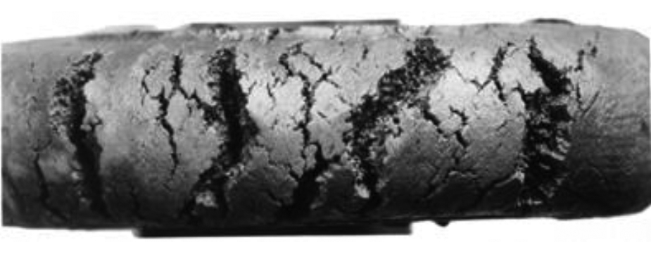
Solid-state sintering is a widespread technique used in the powder metallurgy of ceramics, metals, and superalloys. It is a phenomenon that involves densification of the powder at high temperatures below its melting point with or without the application of external pressure to obtain a consolidated green compact with good strength [2]. This thermal treatment imparts strength and integrity. Sintering consists of three steps—the initial stage when neck formation begins, the intermediate stage when pores interconnect, and the final stage when pores become disconnected thereby forming a consolidated material [3]. Pressure-less sintering involves heating the powder to a high temperature for a long time such that the powder consolidates due to homogenized densification obtaining good green strength. The thermal evolution during pressure-less sintering depends on the inherent thermal properties of the powder such as thermal conductivity and heat capacity. In addition, densification is strongly dependent on the temperatures involved during sintering. These thermal properties are different for the powder as compared to bulk material [4]. Porosity in the unconsolidated powder has a major effect on the thermal and mechanical behavior. As these pores act as thermal insulators, the material in the powder form exhibits different heat transfer compared to a continuum bulk material with no pores. Heat transfer in porous media can occur by conduction through base material, convection from surrounding atmosphere and radiation through pores. Conduction is the dominant process of heat transfer during sintering in vacuum at relatively lower temperatures where radiation is not much [5]. Powder size and pore size also have an effect on the heat transfer. Finer powder has more surface area to volume ratio and hence would have better heat transfer resulting in enhanced thermal conductivity. Thus, it is important to analyze powder mesh size and distribution during preheating cycles as they affect thermal evolution and mechanical properties. In order to obtain homogenization in terms of heating and densification throughout the material, sintering time can take place for several days depending on the size and shape of the product. Hence, such manufacturing processes are time consuming and costly. Based on literature on sintering curves for superalloys (%%0415_OSU_G1%%), the accuracy of temperature predictions can be a determining factor to predict the densification of powder. Even a small variation in temperature prediction with respect to the real case can result in an incorrect densification prediction. Non-uniform temperature distribution, in the preheated component can, results in thermal stresses that lead to cracks near the outer surface as shown in Figure 1.
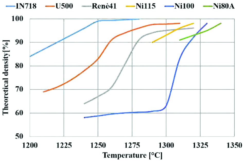
As heat transfer takes place from the surface to core, the surface reaches the desired temperature much faster than the core. This results in a density variation as seen in the graph for superalloys (Graph 1). The surface tends to densify much faster than the powder in the core resulting in significant difference in mechanical properties. Powder consolidation and bonding occurs rapidly near the surface while the core is still unconsolidated and porous even after several hours of preheating. For example, in case of preheating IN718 superalloy powder billet in the temperature range between 1300°C and 1330°C, minute temperature difference between the core and surface can result in large variation in density ranging from 63% to 95%. This variation can lead to non-uniform mechanical properties that adversely affect the performance of the component. Thus, it is important to achieve homogenization throughout the powder component to obtain uniform thermal and mechanical properties thereby eliminating critical defect issues arising due to inhomogeneity.
Prior computational applications explored the possibility of predicting the thermal behavior of a metal undergoing a thermal or thermo-mechanical working cycles. These kind of analyses represent the classical numerical calculation of thousands of processes and could be considered like a standard in the actual state-of-art of FEM models. However, the classical numerical approach may create issues in terms of computational cost and time, especially when long processes are simulated. This severely limits the scope of investigations of critical physical mechanisms. A good help may come from the timestepping techniques, which allow the user to compress the real process time by means of simple mathematical considerations accelerating the temporal behavior of the material. In this case, it is possible to reduce computational time drastically maintaining a good quality of results and coherent physical characteristics of the solution.
The critical part is to explore and acquire proper knowledge to relate mathematical form of parameters within the numerical model to response of the code. It often happens that the governing equation depends on several factors with each one having its own weight inside the formula due to its dependence from linear or derivative forms. It means that a value change of a parameter can produce different effects on the final result of the computation because of different error sensibility of mathematical operators and their coupling.
Szabò [6] investigated the numerical solution of the one-dimensional heat conduction equation by applying Dirichlet and Neumann boundary conditions in order to obtain a good numerical result. The space was discretized by applying the linear finite element method while the theta-method was used for the time discretization. The core of the work was to select theoretically the correct time step size in FEM for the original physical phenomenon to be analyzed.
Tronel and Fichtner [7] focused on timestepping optimization during both coupled and non-coupled thermal and mechanical analysis. The timestepping optimization itself was described with its various possible variants and applied to solve numerical examples. The procedure allows the reduction of computation time by a significant factor when compared to standard uniform timestepping. The study reported in this paper is based on a simulation campaign having the aim of predicting the thermal evolution of a metal powder during a sintering process. This kind of industrial process takes several days to be completed and a quick numerical prediction is often needed to help select the desired process parameters.
The simulation campaign was conducted by using the time-compression method in order to obtain a reduction of calculation time. During the simulation campaign, the influence of different coefficients concerning the heat transport phenomena were studied with respect to accuracy of the numerical result, and the numerical issues arising from the FEM code. The aim of this study is to find the best way to simulate this kind of process without compromising the physics of sintering phenomena.
Heat Transfer Calculation
Heat transfer is the section of science concerning the energy transportation between bodies having a temperature difference [8-11]. This energy transport is classified in three different mechanisms: conduction, convection and radiation and all of them are generally present in a real physical problem [12].
The aim of the calculation is finding the temperature distribution inside the material bodies undergoing to the heat exchange phenomena. The knowledge of temperature distribution within the material may be used to determine the thermal stress. By deriving the conduction equation inside a Cartesian coordinates system and applying the energy conservation criteria to a differential control volume (Figure 2), the temperature distribution in the medium is obtained.
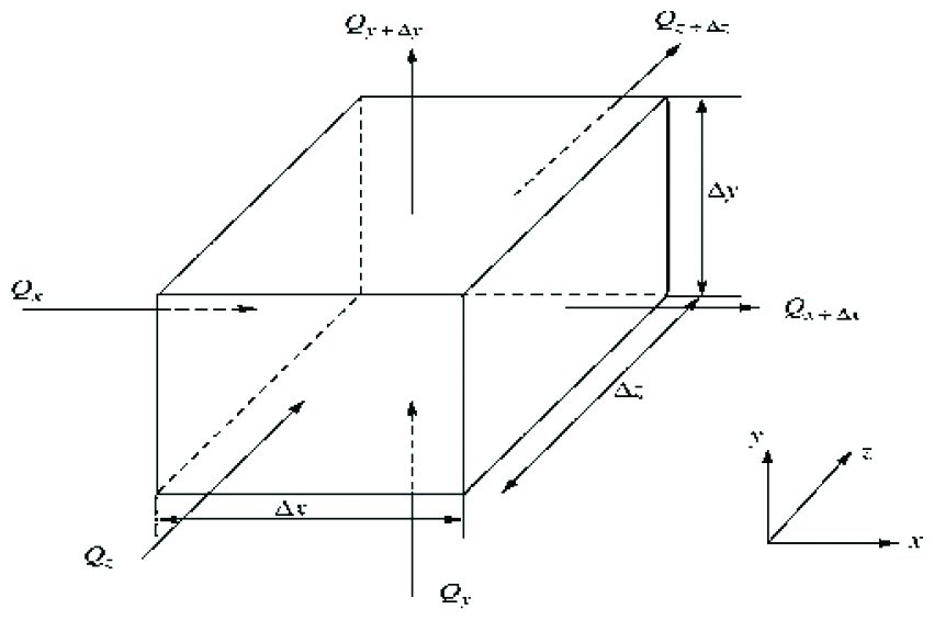
Once this temperature distribution is known, the heat flux at any point within the medium, or on its surface, may be computed by means of Fourier’s law (Equation 1).
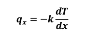
[1]
where k is the thermal conductivity. By applying the Taylor series expansion (Equation 2), limited to first order, to the control volume (Figure 2) it results in the following:
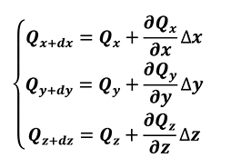
[2]
Considering heat generation in the control volume (Equation 3).
[3]
and the rate of change in energy storage (Equation 4)
[4]
where r is the medium density and cp is the specific heat capacity, it is possible to write the thermal energy equilibrium of the control volume (Equation 5).
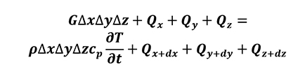
[5]
Considering the Taylor series expansion (Equation 2) the previous equation (Equation 5) can be written as (Equation 6).
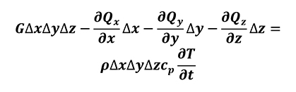
[6]
The total heat transfer in a tri-axial system can be represented as (Equation 7).
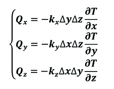
[7]
Considering heat transfer (Equation 7) and control volume, the heat conduction equation for a stationary system in Cartesian coordinates can be expressed as below (Equation 8).
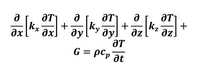
[8]
In the previous equation k is the thermal conductivity of the considered material, which can be expressed as a following tensor (Equation 9).
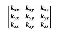
[9]
The previous general form for thermal conductivity can be simplified by means of a one-directional form. This approach is common for such materials in which the thermal behavior is considered like isotropic. The equation below represents thermal diffusivity for isotropic materials (Equation 10).
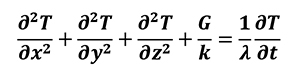
[10]
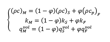
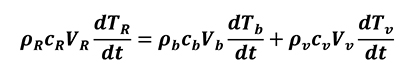
Where thermal diffusivity l=k/rcp. For porous media with isotropic behavior, negligible effects come from radiative transfer, viscous dissipation and pressure work. By assuming the local thermal equilibrium and parallelism of heat conduction between solid and fluid atmosphere, as well as a constant porosity we can write the thermal transport equation for both the solid (Equation 11) and liquid phases (Equation 12).
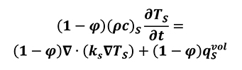
[11]
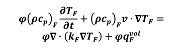
[12]
The subscripts S and F refer to the solid and fluid phases respectively, j is the porosity of the material, c is the specific heat capacity of the solid phase, cp is the specific heat at constant pressure of the fluid phase, k is the thermal conductivity, qfvol is the heat production per unit volume in W/m3[9, 13] and v= jV is the Dupuit-Forchheimer relationship. In this case, it can be observed that there is a linear relation between density and physical thermal properties.
If we consider same temperature for both solid and fluid phase in the previous equations (Equation 11, Equation 12) we obtain the following general equation (Equation 13).
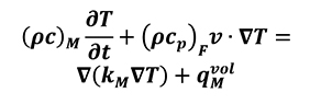
[13.a]
[13.b]
FEM Heat Transfer Analysis
The basic equations and the FE formulation for heat transfer analysis arise from the energy balance equation that can be expressed for isotropic materials as below.
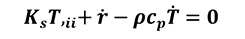
[14]
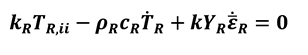
Where Ks is the thermal conductivity, T,ii is the Laplace differential operator for temperature, Ks T,ii represents the heat transfer rate, rcp Ṫ is the heat generation rate and the term represents the internal energy rate. The previous equation (Equation 14) shows the general approach in case of thermo-mechanical analysis in which the heat generation coming from the plastic deformation (Equation 15) has to be considered.
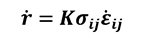
[15]
In the previous equation (Equation 12) K is the heat generation energy coming from that fraction of mechanical work transformed into heat. For metals, this portion is assumed as 90%, while the remaining 10% is consumed by the microstructural changes.
By using the divergence theorem and considering the volumetric integrals, the energy balance equation (Equation 14) can be written as follows:
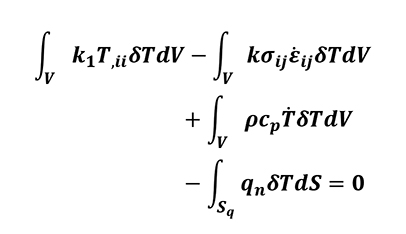
[16]
Where Sq is the boundary surface and qn represents the normal heat flux across that surface:
[17]
The previous equation can be solved only if the boundary temperature field (Equation18) is known.
[18]
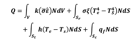
[19]
The first term on the right side of the equation (Equation 16) represents the heat coming from the plastic deformation work. The second term represents the heat coming from radiation of environmental medium, in which s is the Stefan-Boltzmann constant x and is the surface emissivity. The third term is the heat coming from convection phenomenon from the body surface to environmental medium, in which h is the heat convection coefficient. The last term is the heat transferred between bodies in contact [5].
The previous analysis is correct when bulk materials are used. However, for porous media, the energy balance equation has to be defined properly as below (Equation 20).
[20]
Where the subscript R denotes the equivalent quantities of a porous material within a continuum formulation, kR and cR apparent thermal properties derived from the bulk material. By assuming this hypothesis, it is possible to adopt the same mathematical procedure for non-porous materials as for a solid.
The physical behavior of porous material takes place by conduction through rigid base, and convection and radiation phenomena through pores. Depending on the size of pores, the convection can be considered as negligible while the contribution of radiation can be neglected if temperature is low. This signifies that conduction plays a major role.
However, porosity can have complex effects on thermal properties of the material and such aspects are studied extensively by assuming simplified hypothesis.
By assuming heat flow to be unidirectional, pore distribution equal in all directions and thermal properties homogeneous, Im and Kobayashi [14] proposed a linear equation linking the thermal conductivity of powder material to the base bulk material (Equation 21).
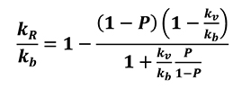
[21]
Here, kR is the apparent thermal conductivity depending on both the volume fraction of pores and the thermal conductivity ratio between bulk material and air inside cavities; kb is thermal conductivity of the base bulk material; kv is thermal conductivity of the pores and P is the porosity of the volume fraction of voids. By introducing the apparent density pR of porous material as well as its specific heat, cR it is possible to obtain the internal energy change relation (Eq. 22)
[22]
p is the density, c is the specific heat, V is the volume and the subscripts R, b and v are related to porous material, base bulk material and pores respectively.
Powder-Bulk Thermal Relationship
As explained previously, this kind of analysis is related to the thermal physical properties of bulk base material as well as powder characteristics. In particular, the major thermal parameters are directly related to density value of powder when the considered material is assumed as isotropic. By following this logic, the simulation campaign was split into two main approaches for thermal analysis. The first one considers the billet as a powder having 70% packing density and a thermal characterization (in terms of thermal conductivity and heat capacity) of the bulk base material. The second one considers the billet as bulk base material having 100% of density and a thermal characterization of the powder. Thermal data of the material for these two density cases was carried out by means of theoretical relationships, considering the following equations (Equation 23) for calculating thermal conductivity and heat capacity of the powder material starting from the bulk base material and directly dependent on amount of porosity [4].
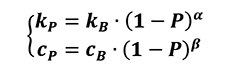
[23]
Where:
- kp is the thermal conductivity of the powder material;
- kB is the thermal conductivity of the base bulk material;
- cp is the heat capacity of the powder material;
- cB is the heat capacity of the base bulk material;
- P is the porosity value of the considered powder material
a and b are coefficients depending on the material.
However, thermal conductivity and heat capacity of bulk material depend on temperature as shown in the following equation (Equation 24).
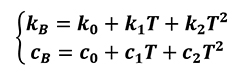
[24]
Where:
- k0 is the thermal conductivity of the bulk material at room temperature;
- c0 is the heat capacity of the bulk material at room temperature;
- k1,k2,c1,c2 are coefficients depending on the material.
Time-Compression Factor Determination
Each simulation was accompanied by the use of different level of time-compression in order to make the process faster by 10, 100 and 1000 times respectively. Each compression factor was obtained by simple mathematical considerations on energy balance equations (Equation 10, Equation 14) for pure thermal case. The Fourier equation (Equation 10) was considered for and simulation objects (Equation 25) and furnace atmosphere (Equation 26) separately.
[25]
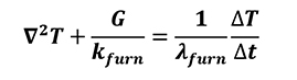
[26]
Where lmat is thermal diffusivity of material when solid simulation objects are considered, while kfurn, lfurn and G are thermal conductivity, thermal diffusivity and convection coefficient of furnace atmosphere respectively.
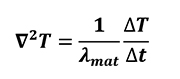
In the case of solid continuum objects, if real temperature variation DTreal is assumed to be equal to simulated temperature one DTsim and Laplace spatial operator D2T is considered as constant (due to constancy of geometries), the Fourier equation (Equation 25) can be written as below (Equation 27).
[27]
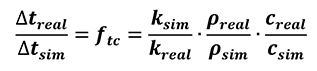
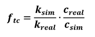
Where is the time-compression factor for simulation. In this way, a linear relation between simulated time and real time of the process is obtained. It is sufficient to change the value of diffusivity parameters inside the numerical code to obtain a speeding of simulated time with a compatible result with respect to standard time simulation. If density is the same for both standard (real) and compressed time (simulation) approach, the equation (Equation 27) can be written as below (Equation 28).
[28]
The equation above (Equation 28) considers thermal conductivity having no dependence of temperature. However, thermo-physical properties of materials in general do have temperature dependence, as shown by thermal conductivity and heat capacity equation (Equation 24).
When the same logic is applied to the furnace atmosphere (Equation 26), it has to be considered that, due to the simulation ambient in which a heating atmosphere is simulated by means of boundary condition for the solid simulated objects, physical variables of furnace medium can be neglected. The only parameter that needs to be taken into account is the convection coefficient G, which regulates the energy flux per time unit. It means that, every time that a specific time-compression factor has to be used, the value of G has to be multiplied by the same factor in order to obtain the same amount of energy going into solid bodies during the simulation.
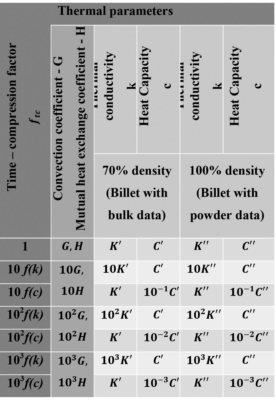
Thus, the time-compression method can be affected by changing k, c and G parameters. Considering that the time-compression method changes the ratio between temperature and time, the effect and the accuracy of results may vary as functions of thermal material properties, which can be constant, linear or quadratic functions of temperature (Eq. 24). Keeping in mind this dependence, the effect of thermal conductivity on accuracy of results was considered in the time-compression approach by using a linear dependence between ftc , k , c and G as shown in the table below (Table 1) which summarizes the thermal parameter set-up for each time compressed simulation.
Case Study
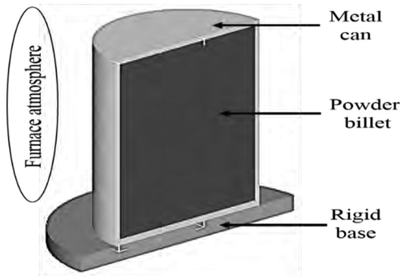
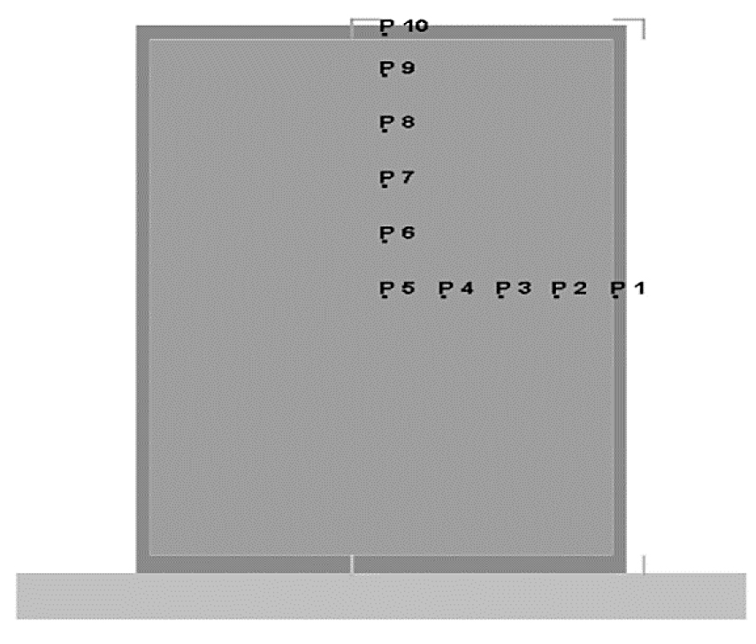
An experimental campaign* was conducted on preheating of a nickel-based superalloy powder with 60 – 80% packing density in order to find the optimal set-up for homogenization. Results were carried out by tracking the thermal evolution of powder with the help of thermocouples placed inside the metal can at different locations, as represented in (Figure 4). To replicate the thermal evolution of superalloy powder during this experimental process, a simulation campaign was carried out using the implicit lagrangian code DEFORM3D™ with a multi-body approach considering the main object (superalloy powder as billet) placed inside a metal can and in contact with a rigid base (Figure 3). The material of the can is assumed different with respect to the rigid base. The main objective of this simulation campaign was to calculate homogenization time required by superalloy powder during the preheating stage with the best ratio between quality of prediction and computation costs. It is well known that long preheating cycles are necessary for superalloy powders due to their thermo-mechanical properties, to achieve homogenization and green strength, especially for further processing involving large aerospace components[1]. In order to verify the capabilities of numerical code, the first approach in simulation was to model the powder like porous material using a continuum solid body having the same density of experimental powder and thermal properties of bulk material. The results of this first approach showed that the code was not able to match the thermal evolution observed during experiments. The reason for this discrepancy can be attributed to the in-built material definition. In fact, the experimental material data (in terms of thermal properties) captures the true physical nature and effects of powder size and distribution throughout the can. Based on this experimental evidence, another approach in which the solid continuum body is modeled like bulk material having thermal properties of powder was considered. This new simulation required to know the thermal conductivity and heat capacity of powder material [4] and, based on experimental data, it was found that the considered superalloy powder showed a linear dependence of thermal properties on density (Equation 23). The results of both 100% and 70% density simulations, in terms of temperature point-tracking in the same positions (Figure 4) of thermo-couples in the experimental test, showed a difference between the two cases with respect to radial (Graph 2) and axial directions (Graph 3). The full density simulation, in which the material has powder thermal properties, matched the thermal evolution of experimental can accurately. Hence, it was considered as the “benchmark” simulation.
The whole simulation campaign was carried out using the same numerical parameters, as below:
- Time step: 5 sec;
- Double symmetry plane;
- Min element size: 0.3 mm
- Max element size: 0.9 mm
- Billet mesh element number: 32770;
- Can mesh element number: 14200;
- Base mesh element number: 11700.
However, it is very difficult to run this kind of simulation in real time, as it requires a very long calculation time (days) with high calculation costs. In this scenario, it was useful to use the time-compression method to significantly reduce calculation time. This means that all simulation objects have to be considered with respect to the time-compression factor equations (Equation 28). Depending on the thermal parameter selected to obtain a proper value, thermal conductivity or heat capacity c of all materials built in the model have to be modified. The same consideration has to be done for the convection coefficient G related to the furnace atmosphere and heat exchange coefficient H between each couple of simulated objects. The relation between these coefficients and time-compression factor is always linear, as shown in the table below (Table 1).
To simplify the simulation campaign chart (Table 1), all thermal parameters were grouped as shown in the following wording (Equation 29).
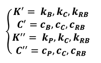
[29]
- kB is the original thermal conductivity of bulk material for the billet;
- kP is the original thermal conductivity of powder material for the billet;
- kC is the original thermal conductivity of the can;
- kRB is the original thermal conductivity of the rigid base;
- cB is the original heat capacity of bulk material for the billet;
- cP is the original heat capacity of powder material for the billet;
- cC is the original heat capacity of the can;
- cRB is the original heat capacity of the rigid base.
Numerical Results and Discussion
The results of all simulations were compared to show the effects and consequences of each approach with respect to the benchmark simulation (experimental result). In particular, the analysis was focused on the error between temperature predictions in the selected points (Figure 4). The final aim is to select the best way to simulate a long process like pre-heating of superalloy powder in few minutes without compromising on accuracy of predictions.
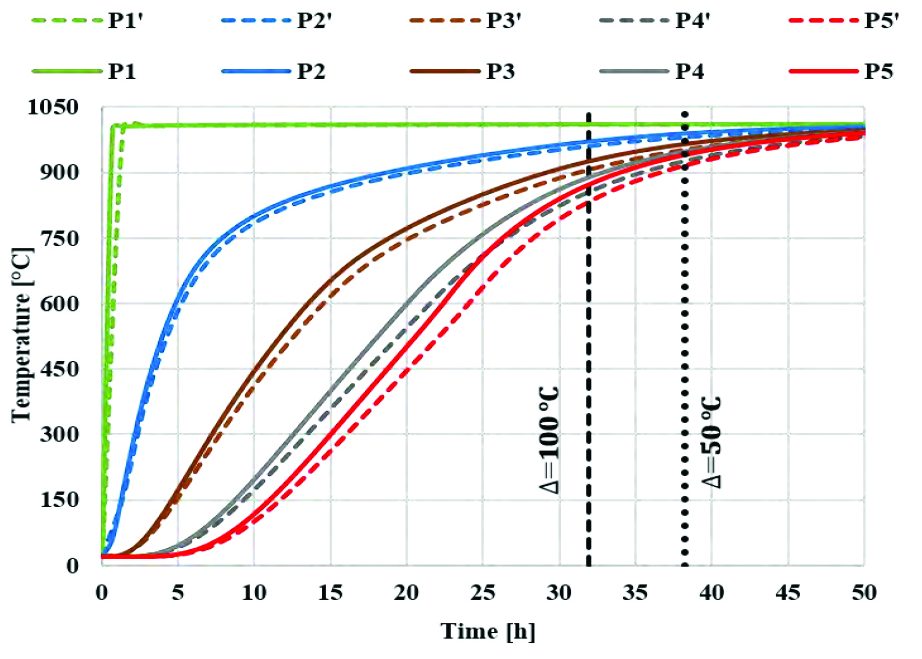
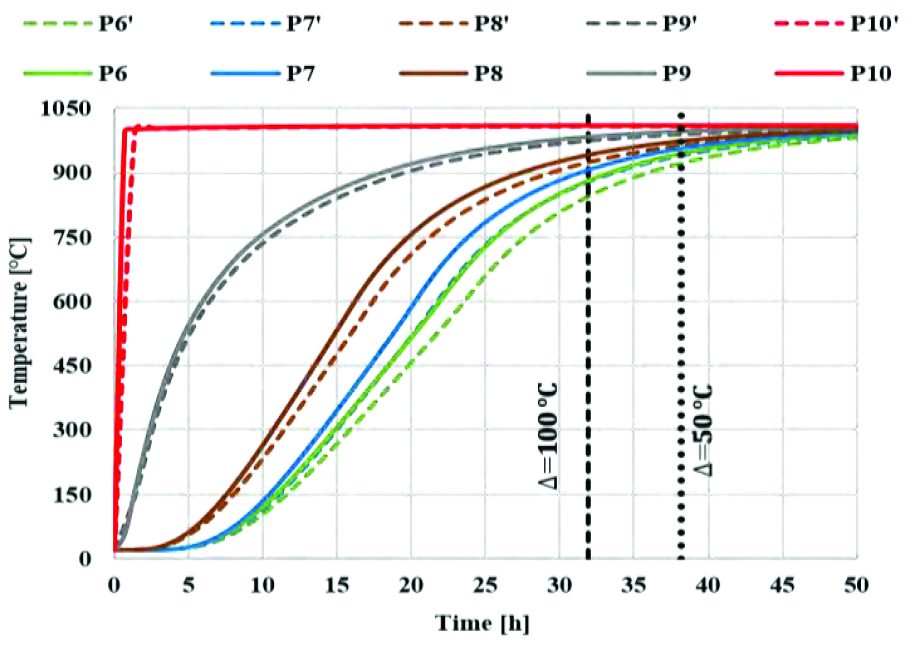
The following graphs represent the temperature evolution along radial (Graph 2) and axial (Graph 3) directions comparing standard time simulations for the case having 100% density with powder thermal data and 70% density with bulk material thermal data. This first comparison (Graph 2, Graph 3) is useful to show the difference in temperature prediction of the billet coming from the use of two equivalent computational logics.
Point-tracking coming from the use of 70% density material with bulk thermal properties differs from curves coming from 100% density material with powder thermal characterization, which represents the most accurate prediction if compared with the experimental plot.
In previous graphs, the vertical reference lines show the time at which temperature difference is 100 °C and 50 °C between the surface and the core of billet, radially (Graph 1) and axially (Graph 2). This can be useful to calculate the homogenization time required for entire billet to reach a desired temperature based on the given application. It must also be noted that thermal behavior of billet depends on the geometry of powder-filled can.
The two approaches can be considered identical according to energy balance equation (Eq. 14) and equation (Equation 23), relating the thermal properties of bulk material to powder and assuming it to be a linear function (with α and β equal to 1). However, thermal relationship between bulk and powder may not always be linear for different materials as the α and β parameters vary between 1 and 2 [4]. This has an effect on temperature prediction.
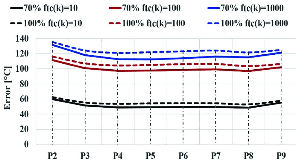
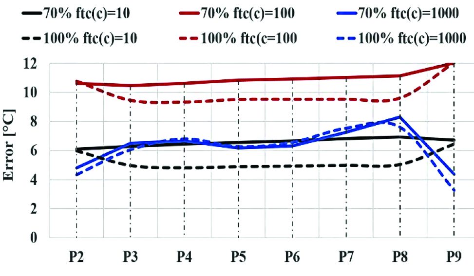
In the case of time-compressed simulations, the results showed a strong relation between thermal parameter used for time-compression factor (Eq. 28) and the accuracy of predictions. The previous graph (Graph 4) shows a variability of the error between 58 °C and 135 °C using time-compression as function of thermal conductivity. The quality of the prediction is similar in both 70% and 100% density simulations. In the same way, the average errors for temperature prediction of each point tracking between the benchmark simulation and the compressed-time campaigns as function of heat capacity were plotted (Graph 5). The results show that the error on temperature prediction is much lower than the previous cases, with a variation between 4 °C and 12 °C and a reduced variability with respect to different values of time-compression factor.
Considering the previous graph (Graph 5), it appears clear that the best quality in temperature prediction is reached by 100% density and compression factor equal to 10 as function of heat capacity. However, the results of both simulations having the maximum time-compression as function of c represent the best compromise between computation costs and quality of prediction.
It appears clear that the time-compression as function of heat capacity provides more accurate results in both 100% and 70% density cases with respect to the simulation campaigns in which the ftc factor is function of thermal conductivity (Graph 4). This can be explained using the energy balance equation (Equation 14) in which thermal conductivity is related to Laplace differential operator for temperature, while heat capacity is related to the derivate of temperature with respect to time. The use of time-compression method does influence the derivate function of temperature in the energy balance equation (Equation 14).
If time-compression as function of c is used, the balance of equation is maintained. However, if time-compression as function of k is used, a different space propagation of thermal wave is obtained as space distribution of temperature has to be maintained in all cases. It can also be correlated to (Equation 24), where thermal conductivity for the powder was assumed to be a linear function of temperature, neglecting the higher order terms.
Finally, considering the calculation time for different cases, the time-compression method allows a strong time reduction, up to two orders of magnitude, as shown in the graph below (Graph 6). A wider range of error with a variability of several degrees amongst the points considered in the billet is observed in case of thermal conductivity, when compared to heat capacity.
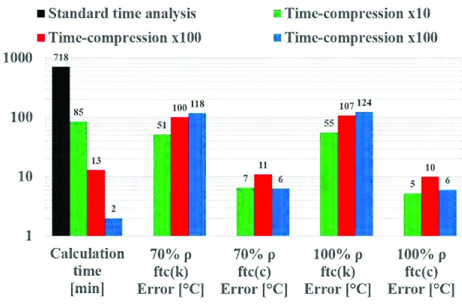
In this panorama, the simulation with 100% density of billet and time-compression factor as function of heat capacity showed the best consistency and minimal error throughout the billet. It must be noted that error in thermal predictions increases with increased time-compression factor using thermal conductivity, while it remains stable when heat capacity is used. This proves that it is possible to carry out, in few minutes, a good prediction of thermal evolution for a densification stage without any limitation in case materials having very different densification curves (Graph 1), where an imprecise estimation in temperature levels could determine the occurrence of defects and, as consequence, the inability to complete the production cycle.
Conclusions
A numerical method to simulate a heating cycle of a powder material by means of a solid continuum model is proposed. The analysis shows the influence of porosity on thermal behavior in the case of two equivalent numerical approaches, one using bulk material with powder thermal properties and the other using porous material with bulk thermal properties. A time-compression technique is developed that reduces the computational cost involved in thermal analysis of such long industrial processes. The influence of each thermal parameter on the prediction of time-compressed simulations is analyzed and a proper setup is obtained with the best ratio between accuracy of results and computational time. This time-compressed approach to thermal modeling can be useful to accurately predict the homogenization time required to reach a particular temperature, along with the powder densification at any given instant based on the application.
References
- Gessinger, G. H., 1984, Powder metallurgy of superalloys, Butterworths.
- Olevsky, E. A., 1998, “Theory of sintering: from discrete to continuum,” Materials Science & Engineering R-Reports, 23(2), pp. 41-100.
- German, R. M., 1996, “Sintering – Theory and practice.”
- Montes, J. M., Cuevas, F. G., Cintas, J., and Muñoz, S., 2012, “Thermal Conductivity of Powder Aggregates and Porous Compacts,” Metallurgical and Materials Transactions A, 43(12), pp. 4532-4538.
- Kobayashi, S., Oh, S. I., and Altan, T., 1989, “Metal Forming and the Finite-Element Method.”
- Szabó, T., 2009, “On the Discretization Time-Step in the Finite Element Theta-Method of the Discrete HeatEquation,” Numerical Analysis and Its Applications, S. Margenov, L. Vulkov, and J. Waśniewski, eds., Springer Berlin Heidelberg, pp. 564-571.
- Tronel, Y., and Fichtner, W., 1999, “Optimal Time Stepping in the Thermo-mechanical Finite Element Simulation of IGBTs Modules,” Technical Proceedings of the 1999 International Conference on Modeling and Simulation of Microsystems Chapter 8: Numerics, Algorithms, pp. 334 – 337.
- Sukhatme, S. P., 1992, “A Text Book on Heat Transfer.”
- Bejan, A., 1993, “Heat Transfer.”
- Holman, J. P., 1989, “Heat Transfer.”
- Incropera, F. P., and Dewitt, D. P., 1990, “Fundamentals of Heat and Mass Transfer.”
- Lewis, R. W., Nithiarasu, P., and Seetharamu, K. N., 2004, “Fundamentals of the Finite Element Method for Heat and Fluid Flow.”
- Bejan, A., and Nield, D. A., 2013, “Convection in porous media.”
- Im, Y. T., and Kobayash, S., 1986, “Coupled thermoviscoplastic analysis in plain-strain compression of porous materials,” Advanced manufacturing processes, 1, p. 269.


 general practice for CQI-9 and AMS2750E")


 steels")
