


Surface metrology parameters represent an important class of design variables, which can be controlled because they represent the DNA or fingerprint of the whole manufacturing chain as well as form important predictors of the manufactured component’s function(s).
Existing approaches of analyzing these parameters are applicable to only a small subset of the parameters and, as such, tend to provide a narrow characterization of the manufacturing environment. This article presents a new machine learning approach for modeling the surface metrology parameters of the manufactured components. Such a modeling approach can allow one to understand better and, as a result, control the manufacturing process so that the desired surface property can be achieved while manipulating the process conditions. The newly proposed approach uses a fuzzy-logic-based-learning algorithm to map the extracted process features to the areal surface metrology parameters. It is fully transparent since it employs IF … THEN statements to describe the relationships between the input space (in- process monitoring variables) and the output space (areal surface metrology parameters).
Furthermore, the algorithm includes a ridge penalty-based mechanism that allows the learning to be accurate while avoiding over-fitting. This new machine-learning framework was tested on a real-life industrial case study where it is required to predict the areal parameters of a manufacturing (machining) process from in-process data. Specifically, the case study involves a full factorial experimental design to manufacture 17 steel bearing housing parts fabricated from heat-treated EN24 steel bars. Validation results showed the ability of this new framework not only to predict accurately but also to generalize across different types of areal surface metrology parameters.
1 Introduction
Surface metrology, defined as the science of measurement of small-scale characteristics (such as amplitude, spacing and shape of features) in manufactured parts [1], forms an important part of the manufacturing processes for two main reasons. The first relates to the fact that surface metrology can be thought of as the fingerprint of the whole manufacturing chain. This fact can be used for control of the manufacturing process [2, 3]. The second reason is that surface metrology can directly correlate with the manufactured components function. Such information is useful for quality assessment and function prediction.
Predicting the quality or how a manufactured component will function is particularly valuable in helping to meet today’s ever tighter budgetary and time constraints as well as the drive for right-first-time production of materials [4]. Indeed, a mechanism for controlling the surface metrology parameters can represent a valuable asset as evidenced by the plethora of research studies that have sought to design algorithms for this purpose [1, 5, 6]. However, before such a control can take place, a mapping from the process conditions to the surface metrology variables must be found. Such a mapping has formed the topic of many research studies for several decades as will be discussed in the next section. The majority of these research studies focus on very simple mappings typically involving the creation of a limited list of input features from the process data. A data model is then found to map these features to selected surface metrology parameters (usually profile parameters).
One notable example is the prediction of the surface roughness heights (Ra) from process conditions [5-7]. It should be noted, however, that these existing studies have mainly focused on predicting the profile parameters, and the application of modeling algorithms for predicting areal parameters, which are arguably more important, is limited [8]. The areal parameters provide a characterization for the full 3D surface of the manufactured part and have been shown to be more descriptive of the surface as well as being better related to its function [8]. Therefore, mappings from process conditions to areal parameters can provide better value for the manufacturing process. This research study will therefore mainly focus on the modeling of the areal surface metrology parameters.
Existing research studies also typically focus on very small subsets of areal parameters while neglecting the others. They also tend to derive coarse scale features extracted from the process data [9, 10]. However, as discussed in [5], many areal surface metrology variables can correspond to a particular function, and, as such, it is often imperative these areal parameters be combined in a systematic way for function prediction. The surface metrology variables can vary in a very different and sometimes unpredictable manner; an approach formulated for predicting one areal parameter might not be applicable for predicting another areal parameter.
As the algorithms hitherto developed have only been validated on one or two areal parameters, it is difficult to make a concrete statement on how such modeling approaches perform across the many areal parameters. Consequently, validating the published algorithms on the other areal parameters (which may perhaps be of equal or more importance depending on the use of the variable) may prove to be problematic.
The study in this article proposes a new framework to predict areal surface metrology parameters based on features extracted from process conditions. The proposed approach is shown not only to generalize across unseen data, but is also robust enough to be utilized for all the 24 areal surface metrology parameters on which the proposed approach is tested.
To validate the developed algorithms, a full factorial experimental design was carried out to manufacture 17 steel bearing housing parts as a case study. The sparse and highly uncertain multidimensional data obtained during this case study represent real manufacturing processes where components are manufactured in low volume. Therefore, the main contribution of this article is the development of a modeling methodology that can generalize to a large number of manufacturing variables using a limited quantity of data.
The details of the experimental design as well as process conditions are discussed in Section 3. The proposed framework presents methodology that can aid the drive toward manufacturing automation and data exchange [11]. The review paper by [12] describes state-of-the-art in terms of algorithms, industry uptake, and investments across a wide-range of manufacturing industries. For different materials and manufacturing processes, machine learning approaches, such as artificial neural networks, have also been developed with limited experimental data for predictive modeling of properties of manufactured components [13].
The properties of the components can be dictated by the properties of the material, mechanical or microstructural, but also via surface metrology parameters within a synergetic framework. There is a plethora of applied research works relating to the causality between process and material data and mechanical and microstructural properties, but there is little work on such causality with respect to surface metrology parameters. This holistic approach should improve our understanding of how the final properties of manufactured components may be optimized for right-first-time production.
The remainder of the article is organized as follows: Section 2 presents a detailed literature review of existing techniques, which have been used for mapping process conditions to surface metrology variables. The section details the strengths and weaknesses of these approaches to the overall manufacturing informatics system. As already mentioned, Section 3 provides a detailed description of the experimental procedure for which the data has been derived. Section 4 discusses the proposed interpretable fuzzy-based machine learning approach for the surface metrology informatics system. Section 5 presents and discusses the results while Section 6 provides the conclusion, which can be drawn from the studies conducted from the paper as well as providing suggestions for future research.
2 Existing literature
The book by Whitehouse [1] may perhaps be described as the most important piece of literature where the use of surface metrology in manufacturing for function prediction and quality control is perfectly detailed. The book forms the foundation of many research studies, which have investigated the use of surface metrology components to predict manufactured components function and consequently to control the manufacturing process. Controlling the manufacturing process is typically achieved by the manipulation of the process parameters. To achieve such a control framework, it is apparent that a model indicative of how the process parameters affect the surface metrology parameters must be identified [14]. Such a mapping framework has been the subject of many research studies as already discussed in [5, 6].
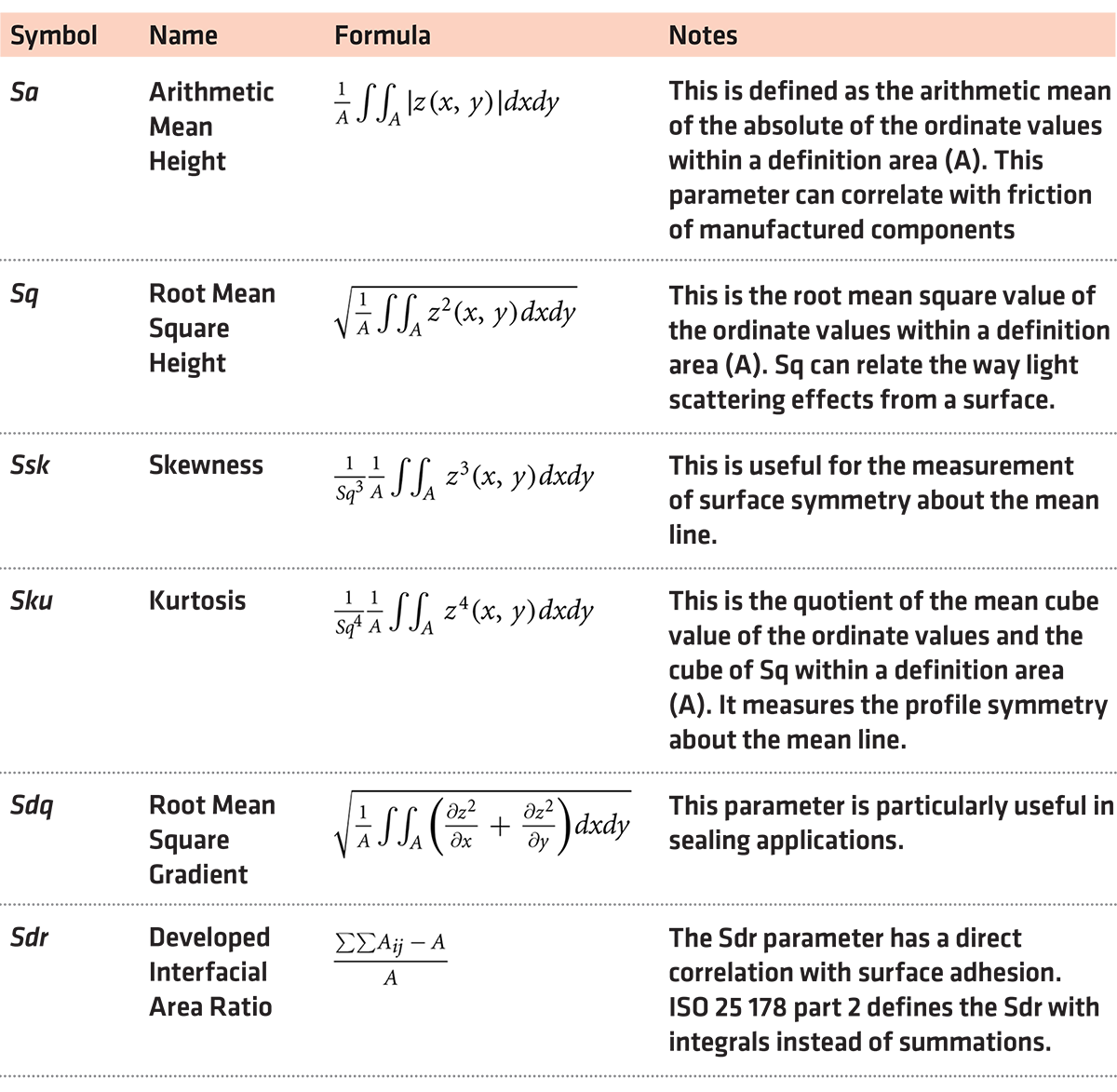
Surface profile parameters account for the majority of surface metrology variables used for understanding the manufacturing chain. Of the profile parameters defined in the ISO standards [15], the surface height (Ra) is the most widely used because its derivation is simple, fast, and its meaning is widely understood by manufacturing technologists. For example, a high value of Ra indicates a visually rougher surface. Predicting the Ra accounts for the majority of the surface profile predicted variable studies. Some of these studies include the prediction of surface roughness parameter (Ra) for a computer numerical con- trolled (CNC) milled surface using linear regression [16] and the assessment of surface roughness using time and frequency domain features for a polished surface [17]. In particular, the studies conducted in [18] have shown that the Ra strongly correlates with the mean and root-mean-square (RMS) of the vibration signals for the polishing process.
However, one of the main limitations of the approach is that predicting the Ra may not be sufficient to fully characterize the manufacturing informatics system. This is because the Ra value is very simplistic and may not account for the variation across the surfaces [17]. One solution to this, which has been proposed in the literature, involves creating a distribution of Ra values, but this has not been widely adopted by both academia and industry perhaps due to the complexity involved [19]. A better and recent approach relates to characterizing the full surface as opposed to using profile parameters. This recent approach is known as the areal surface, and it is the main subject of this article.
One of the most prominent studies in attempting to predict the areal surface parameters relates to the prediction of the Sa parameter for a rotating machined process from process variables as included in [19]. The areal parameters characterize the full 3D surface and have been standardized in the ISO25 178 documents [20]. These documents contain a comprehensive industry standard areal parameters. The parameters as well as their use are shown in Table 1. Many of the algorithms formulated for the prediction of areal surface parameters have only been applied to one or two of the areal parameters [8]. Validation of such approaches on the parameters on which they have not been tested may not be feasible. This article presents a fuzzy modeling approach for the prediction of surface area metrology parameters.
The proposed approach is tested on 24 areal parameters in order to show the proposed approach can be generalized across the various surface metrology parameters. The paper in [21] provides an excellent overview of the use of fuzzy models in areal surface metrology predictions. Fuzzy logic systems provide a unique modeling approach of leading to interpretable but non-linear input/output mapping when predicting the surface metrology parameters. Manufacturing systems are in the middle of a revolution where different components and stages of the manufacturing process are increasingly becoming “intelligent.” This intelligence stems from the fact the many components involved in this process are increasingly able to intercommunicate from upstream to downstream. This special ability is embedded in the concept of Industry 4.0, which references the fourth industrial revolution in which machine components and processes are equipped with cyber-physical capabilities and are thus capable of tuning their process conditions in response to feed- back from the environment and other manufacturing conditions. The promise of Industry 4.0 is well discussed in [22]. Surface metrology represents a key enabling component of this revolution as surface metrology parameters play a key part in the inspection of manufactured components. The surface metrology parameters can provide insights for online decision making in a cyber-physically connected system. The Ra, for example, is a design variable, and it is typically required to not exceed a particular limit for the manufactured component to function as expected.
3 Experimental design
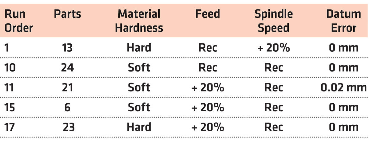
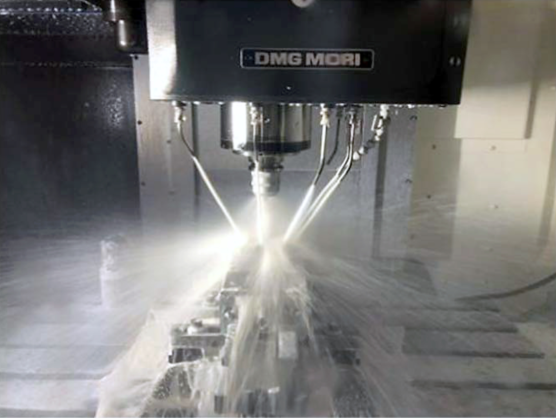
A full-factorial experimental design (see Table 2) was performed on a steel bearing house [22]. The CAD model of the product to be manufactured is shown in Figure 1a. Using a Vecstar furnace, the material blocks (steel EN24) were heat treated to approximately 845°C (Figure 1b) and then quenched in oil so they can be hardened. The next step involved tempering at the selected design temperatures. Temperature gradients and variations during both heating and tempering were also measured using high-temperature thermocouples. The surface hardness measurements of the blocks were obtained using a Rockwell device. The treated product was then machined (Figure 2) using a DMG MORI NVX 5080 3-axis machine with variable controlling factors to arrive at the final manufactured component. During the machining process, process data, such as vibration data, were measured along the three main axes of the work-piece. In particular, vibration data were obtained using an accelerometer sensor placed on the spindle, which were then logged using LabView SIGNAL Express Software.
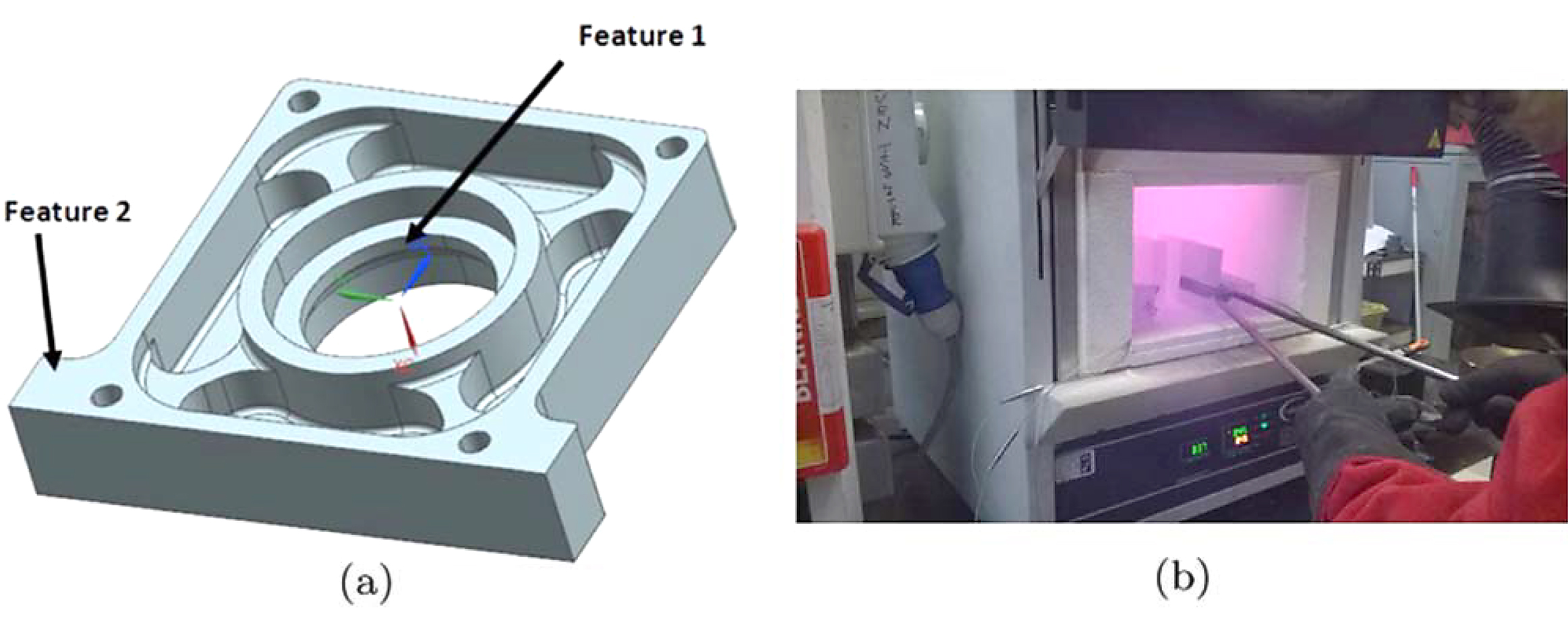
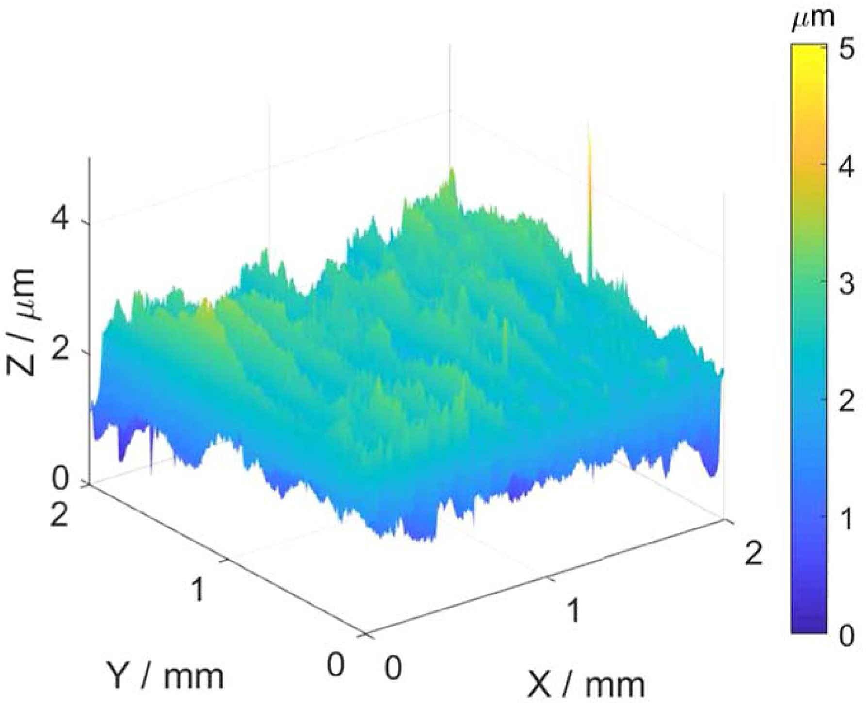
The areal surface measurements were obtained using an ALICONA interferometric instrument. Two surface measurements were obtained per part resulting in 34 measurements in total. The features mea sured per part are shown in Figure 1a. This instrument records the height (z) at sampled locations (x, y) with uniform sampling and a sampling interval of 10 μm. The instrument measures the raw surface metrology data and preprocessing is needed to obtain the standardized surface metrology data. The procedure for obtaining the standardized surface metrology data is shown as follows.
1. Obtain the primary surface by the application of the S-Filter on the real surface. The S-Filter used is the Gaussian filter, and the standards recommended in the ISO 16 610-21 document [23] have been followed. For example, the wave- length of the S-filter is taken to be 15 times the sampling interval (150 µm).
2. If necessary (depending on the result obtained above), perform further surface filtering to obtain the scaled limited surface. It should be noted that this stage is entirely determined by expert knowledge.
3. Specify the evaluation area which is taken as five times the selected wavelength (750 μm).
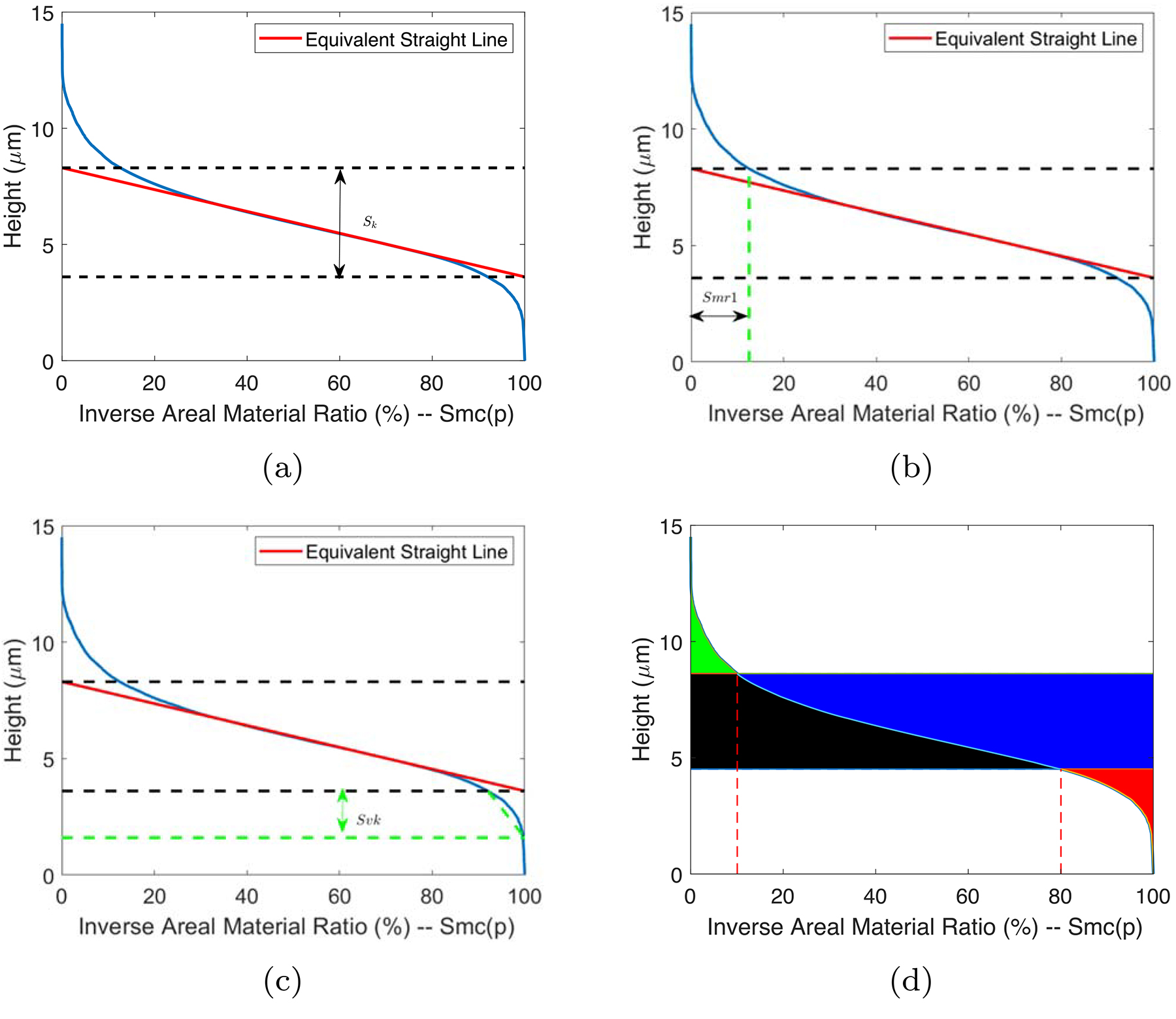
4. Obtain the reference surface and calculate the parameters as described in Figure 3.
A sample of the areal surface metrology measurements obtained following the procedure above is shown in Figure 4.
4 Proposed fuzzy modeling approach
Fuzzy logic represents an extension of bivariate logic and was introduced in 1965 in Zadeh’s seminal paper [24]. Since then fuzzy logic systems have found applications in a variety of domains including biomedicine [25], process control, manufacturing [26], and aerospace systems. The use of fuzzy systems in these applications offers a unique advantage of being able to model non-linear systems in an interpretable manner. The interpretability comes from the fact that a fuzzy logic system is a rule-based system, and the rules are similar to the natural language of humans. These rules also allow for the incorporation of expert knowledge, which can be valuable for the analysis of complex systems. Central to fuzzy logic systems are the fuzzy sets.
Fuzzy sets extend conventional sets in that they can provide to what extent an element belongs to a particular set. Mathemetically, a fuzzy set (type-1), A, may be expressed as follows:
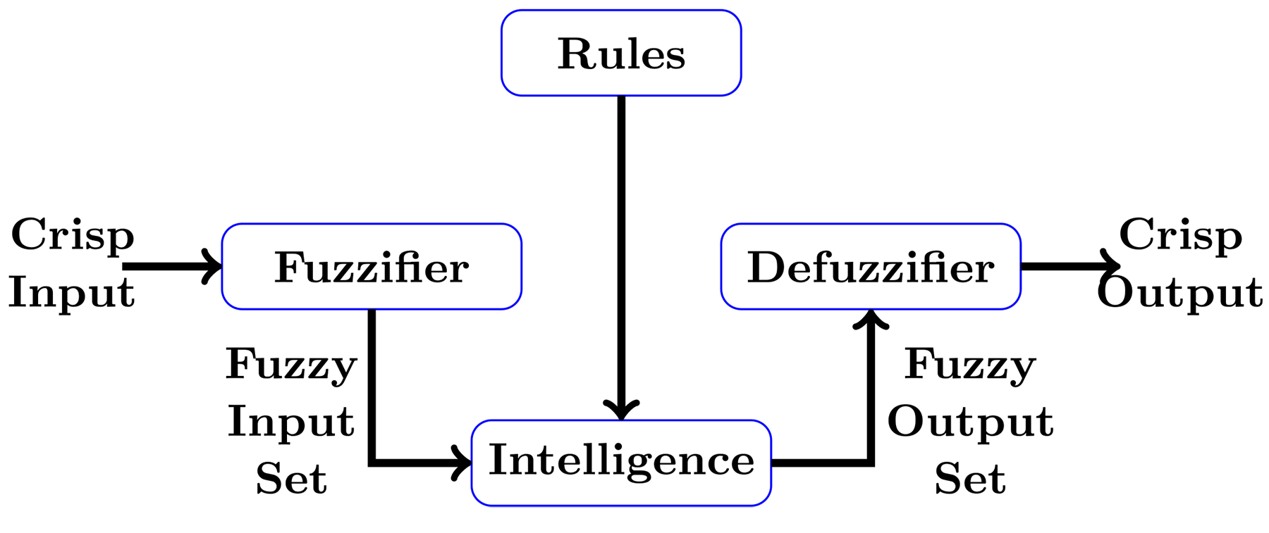
![]() where μA(x) is the membership degree of the fuzzy set of an element x in the Universe of discourse X,0 < μA(x) < 1. The fuzzy logic system (FLS) can be considered to be a mapping from the input space (defined as X) to the output space (defined as Y) (Figure 5). Such a mapping can be formulated by the following equation:
where μA(x) is the membership degree of the fuzzy set of an element x in the Universe of discourse X,0 < μA(x) < 1. The fuzzy logic system (FLS) can be considered to be a mapping from the input space (defined as X) to the output space (defined as Y) (Figure 5). Such a mapping can be formulated by the following equation:
 where ŷ is output of the fuzzy logic system, φj(x) represents the degree of validity for the jth rule (for a total number of c rules) for an input x ⎣ RN× φj(x) represents the normalized firing strength of a particular input in each input space. The nature of λj is what determines if the fuzzy system is of the Mamdani or of the Takagi Sugeno Kang (TSK) type. For the Mamdani type, λj represents the output/consequent fuzzy set of the jth rule while for the TSK type, λj represents a linear function (λj = ax + b).
4.1 Identifying Fuzzy Models
As discussed in the preceding section, the fuzzy model can be thought of as a nonlinear interpretable mapping from the input space to the output space. The fuzzy system is parameterized (the fuzzy sets can be represented by parameters) and such parameters can be learned from the data obtained from the system to be analyzed via fuzzy logic. There exists a plethora of approaches for identifying the parameters of the fuzzy logic system such as optimization of the cost function via gradient descent and iterated re-weighted least squares [27]. As the goal of this article is to develop an approach that can generalize across the different areal parameters, it is imperative that a robust framework be found. Consequently, the proposed algorithm development follows a number of steps as discussed in the preceding sections.
4.2 Fuzzy Modeling Approach
The fuzzy model used here is of the Mamdani type because it can be shown to represent the most transparent of fuzzy models. The block diagram for the process of obtaining the fuzzy model from data is shown in Figure 6.
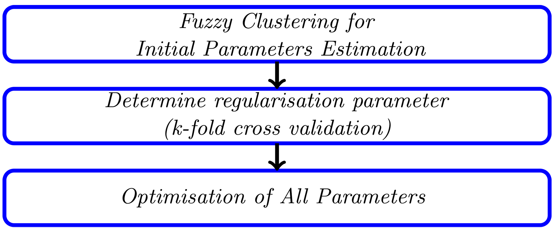
The first step involves the use of fuzzy c-means data clustering of the product space, which provides an initial good guess of the parameters of the fuzzy model and will later be optimized. As shown in [26], such an approach can help in preventing the optimization algorithm from being stuck in a local optima. The number of clusters determines the number of fuzzy rules in the trained fuzzy models. To determine the optimal number of fuzzy rules (which is the same as the number of clusters), a crude search was carried-out to find out the region where the optimal number fuzzy rules is. The authors found that for very large number of fuzzy rules, the algorithm overfitted on the hold-out set, and this gets progressively worse as the complexity of the model increases. The search for the optimal number of fuzzy rules was thus limited to between 2 and 12. The second step involves determining the regularization parameter. This step involves defining a cost function — a penalized root mean square error (RMSE) defined by the following equation:
 where f(X, β) represents the output of the fuzzy system, y is the vector representing the output data and λ is a penalty term that penalizes for large values of the fuzzy model parameters. The value of λ is determined via a K-fold cross validation using the following steps:
Algorithm 1: K-fold cross validation algorithm for determining the regularization term
1. Divide the training data set into K-folds. Note that there is a 70%-30% split in training data to testing data. This resulted in a training data of 24 data points. The value of K was chosen to be 4 which means there were 6 data points per fold.
2. From 10-2 to 106 (on the log scale), select a particular λ and train the fuzzy model on the three folds and test on the remaining one fold. The approach is repeated until when all the data folds have been tested. Record the λ value and corresponding RMSE.
3. Zoom in on the λ values and find the λ values with the lowest error (RMSE) and repeat procedure 1-2 if necessary.
4. Select the fuzzy model with the lowest RMSE (without the penalty term) and record the value of λ.
It should be noted that steps 2 and 4 above involve a training procedure which involves finding the parameters, which minimize the error function as defined in Equation 3. The procedure by which this has been done in Algorithm 2 is based on the scaled conjugate gradient algorithm.
Algorithm 2: Scaled Conjugate Gradient algorithm for finding the optimal parameters
Given the objective function of Equation 3, the parameters of the fuzzy models are obtained via the scaled conjugate gradient descent algorithm. The fuzzy sets for both the antecedent and the consequent variables are assumed to be defined by Gaussian membership functions with two parameters, ![]() v and σ correspond to the center and spread of the membership function. The output of a Mamdani fuzzy system is given by the following equation:
v and σ correspond to the center and spread of the membership function. The output of a Mamdani fuzzy system is given by the following equation:
 where x represents the jth input for a total of n inputs and c fuzzy rules. The derivative of the antecedent and consequent parameters are given by the following equation:
 where θlij is the lth parameter of the jth antecedent of the ith rule. for j = 1, 2, ¼ ,n, i = 1, 2, ¼ c, and l = v, σ. For each parameter, it can be shown that their derivatives with respect to the center and spread of the membership functions can be given by the following equations:

 The derivative with respect to the consequent parameter is given by the following equation:
 where βi is the consequent parameter of the ith rule. It should be noted that N represents an unnormalized Gaussian function. F is a vector representing the firing strengths across all the rules and 1 is a vector of ones. It is worth emphasizing that the scaled gradient descent algorithm was used in this article. At iteration k, the parameters are updated as follows:
![]() P is the vector of parameters, α is the step size, and d is the search direction. ψk = αkdk is given as follows:
P is the vector of parameters, α is the step size, and d is the search direction. ψk = αkdk is given as follows:
 where H is the Hessian that can be approximated as discussed in [27]. It is worth emphasizing that Equation 3 includes a loss function, which can be used to control the interpretability of the elicited fuzzy model. The center of sets defuzzification method was employed in this research, but the proposed approach extends easily to other defuzzification methods.
5 Results
5.1 Data
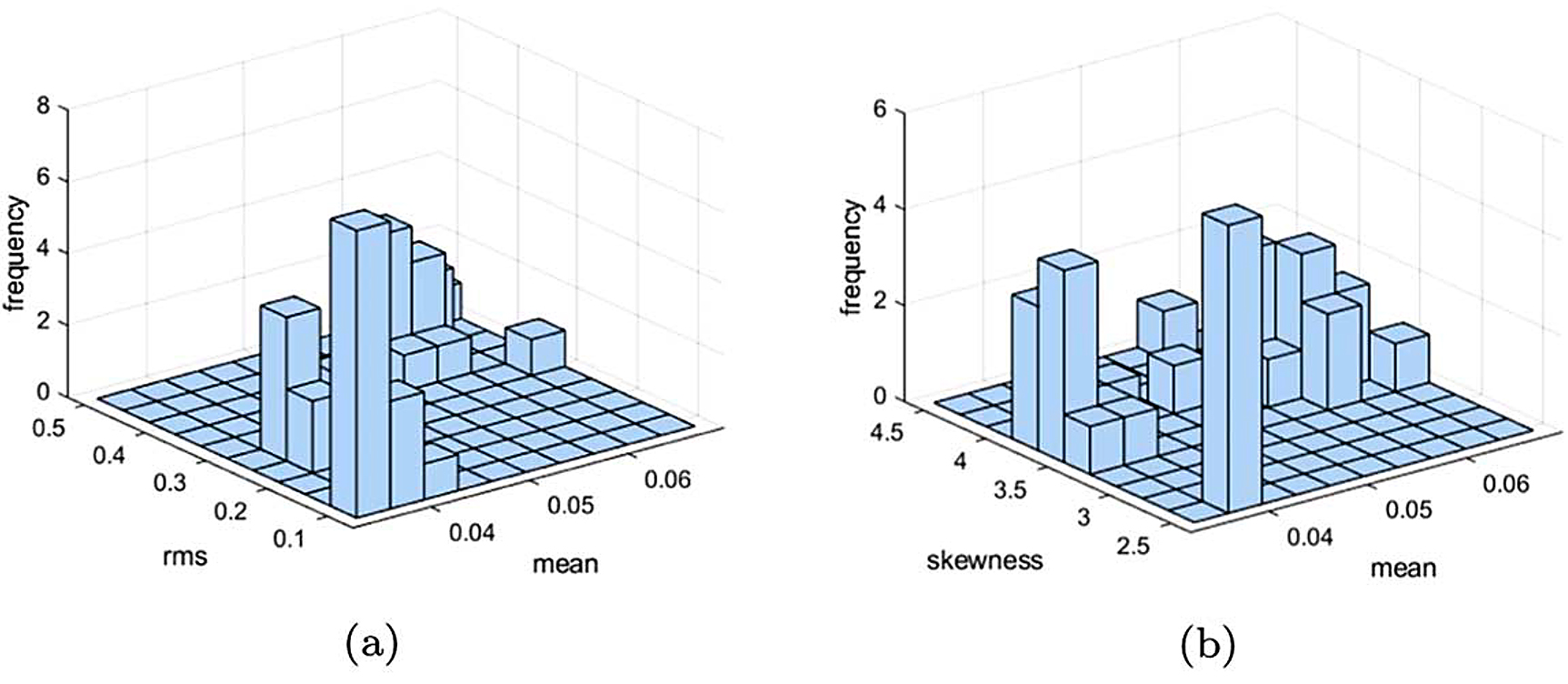
The datasets used in this research study are the surface metrology data (an example is shown in Figure 4) and the process vibration data. The vibration dataset is a time series data sampled at a frequency of 10KHz. Sets of vibration data in the x, y, and z directions were obtained per feature in each of the parts. From the vibration data, feature extraction was performed. The features extracted included time and frequency domain features (for example mean [10], root mean square value [17] and the Fourier transform frequency components). A total of 206 features were obtained from the vibration data. A distribution of the vibration data as well as selected input features shown in Figure 7 indicates the data is sparse and multidimensional.
The 24 areal parameters from the surface metrology were also obtained using an in-house software developed by the authors. The procedure for deriving the parameters are as outlined in the ISO standard as well the studies performed in [20, 28].
It is worth emphasizing that the modeling problem is challenging because of the high dimensionality and sparseness of the data points. Specifically, there are 34 data points in all (25 training data points), which points to the fact that it is easy to overfit on the training data [26]. This phenomenon is representative of many manufacturing processes (such as in the manufacture of aerospace components) where parts are manufactured in low volume. It would be interesting to investigate how the proposed approach performs in this challenging modeling problem. It should be noted that a penalized error function coupled with K-fold cross validation is proposed for the modelling problem as discussed in section IV. There is a 70%- 30% split between training and testing data sets. This split was performed after a random sampling of the full data set.
The performance metric used for evaluating the developed models is the RMSE. The 206 features were extracted from the raw vibration data. New deep learning approaches make it possible to use raw time-series data in the modeling problem as shown in [29]. This line of thought was not pursued further because this may not be feasible for cases of low volume manufacture such as the one considered in this paper.
5.2. Linear Regression Modeling
Linear regression modeling is the work-horse of modeling in manufacturing. To test the proposed approach on other modeling problem, linear regression is chosen as a benchmark so the results obtained from the proposed approach can be compared. The linear regression modeling is given by the following equation:
![]() where X represents the design matrix and β the corresponding parameters. ε represents a zero-mean Gaussian noise. For a sum of error square cost function, the solution to the optimization problem is given by the following equation:
where X represents the design matrix and β the corresponding parameters. ε represents a zero-mean Gaussian noise. For a sum of error square cost function, the solution to the optimization problem is given by the following equation:
![]() It is worth noting that, as there are significantly more features than data points, the linear regression modeling problem will be overdetermined and will result in overfitting on the modeling problem. This was indeed the case when a linear model was performed on the training data. These results are shown in Figure 8.
It is worth noting that, as there are significantly more features than data points, the linear regression modeling problem will be overdetermined and will result in overfitting on the modeling problem. This was indeed the case when a linear model was performed on the training data. These results are shown in Figure 8.
As can be seen from the results of Figure 8, the linear regression model fits the training data perfectly but does not generalize well to unseen data (as can be noted form the testing data set performance). To allow for better generalization to unseen data, the linear regression cost function can be penalized as given by the following equation:
![]() where λ is called the ridge parameter whose function is to penalize for large weights. As already mentioned, the penalty term (λ was determined by K-fold cross validation) as described in Section 3. The penalized linear regression (ridge linear regression) results is as shown in Figure 9.
where λ is called the ridge parameter whose function is to penalize for large weights. As already mentioned, the penalty term (λ was determined by K-fold cross validation) as described in Section 3. The penalized linear regression (ridge linear regression) results is as shown in Figure 9.
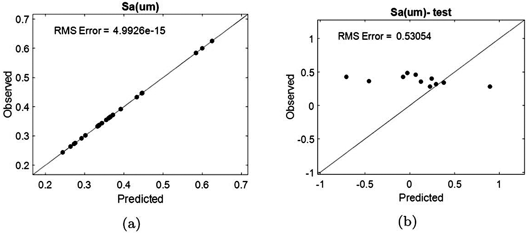
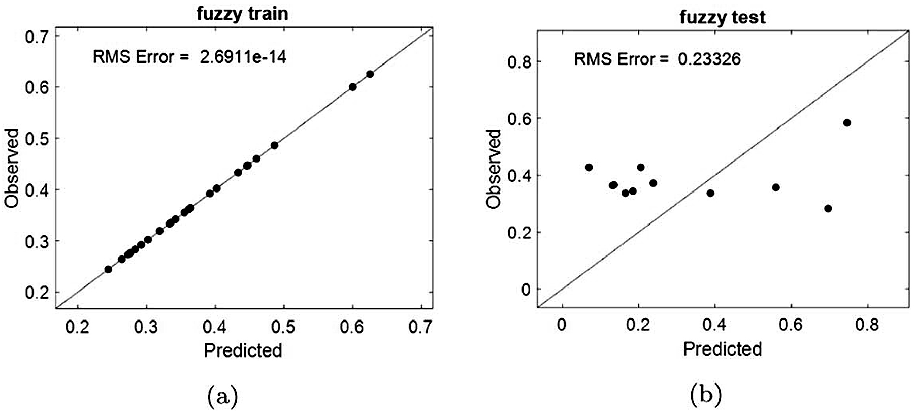
As can be seen from Figure 9, although the results of the testing datasets are more generalizing when compared with ordinary linear regression results, the training data set is significantly much worse. This is as a result of the fact that the ridge parameter is able to find a compromise between the best training results (in the linear sense) and the best validation results (in the linear sense). The results suggest that a non-linear model is required to obtain a good mapping of the process parameters. It is for this reason that the Mamdani fuzzy model is first considered as discussed in Section 3. The first Mamdani model considered is not inclusive of any penalty term that has already been explained can result in overfitting of the training model. Such a result is similar to the ordinary regression result (shown in Figure 8). The fuzzy modeling result without any penalty term is shown in Figure 10.
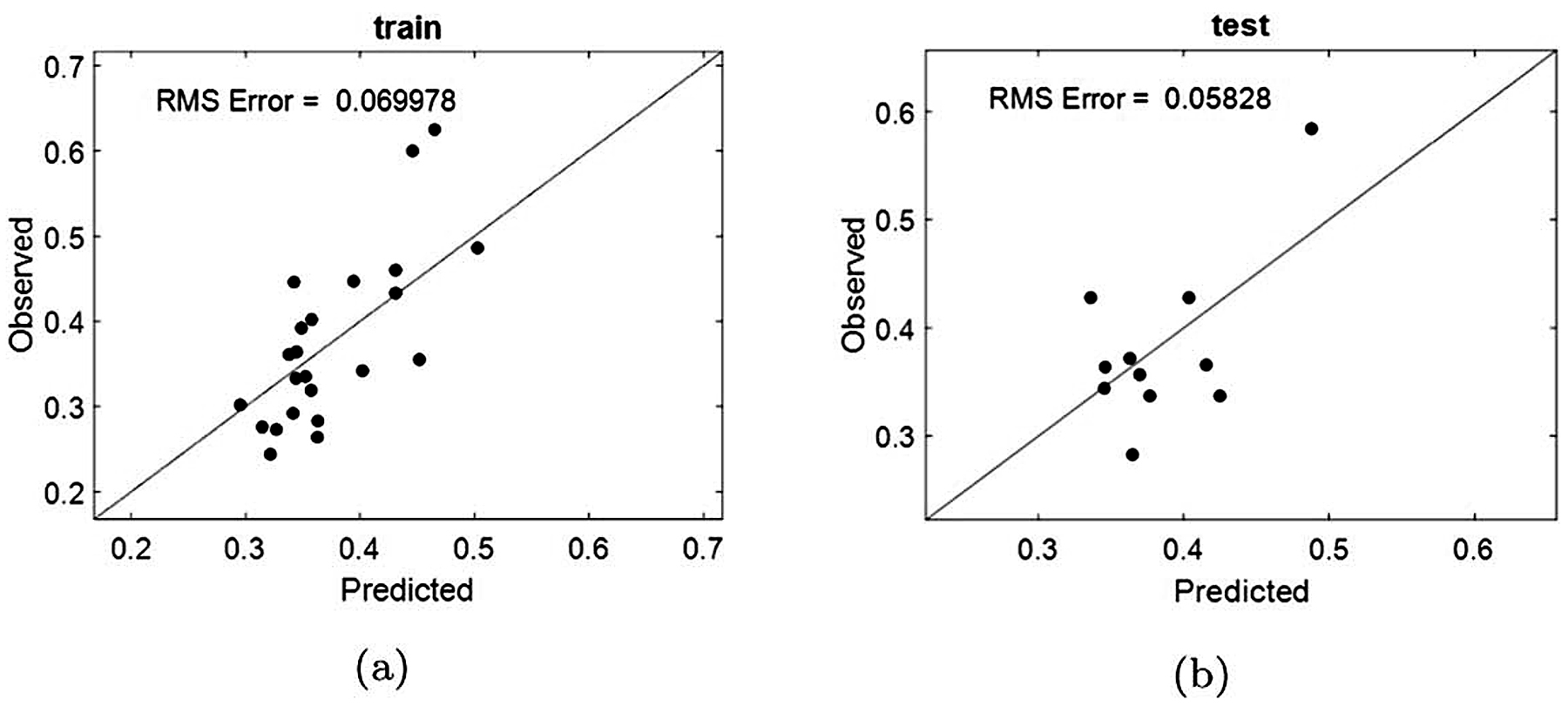
To allow for better generalization, the same ridge linear regression training procedure (discussed in Section 4) is also followed to train the Mamdani fuzzy model. The results of the ridge Mamdani fuzzy system is shown in Figure 11. We have called this approach the ridge Mamdani fuzzy modelling approach to emphasize its capability to penalize for large fuzzy weights in order to improve generalization performance.
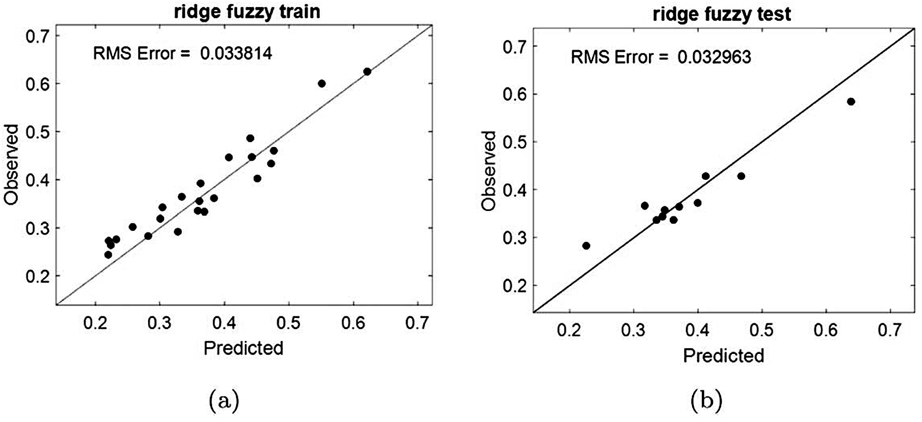
As can be seen in Figure 11, the ridge fuzzy modeling framework provides a much-improved performance and is able to map the process features to the surface metrology parameters. The result shown in Figure 11 can be replicated across all the other areal surface metrology parameter, which indicates the proposed modeling methodology predicts with accuracy regardless of the parameter of interest. Tables 3 and 4 respectively show the performances of the linear/ridge regression method and the proposed fuzzy approach in predicting 24 areal parameters. The results from these tables indicate the proposed approach is able to generalize across different areal parameters and provides consistent as well as robust modelling results.

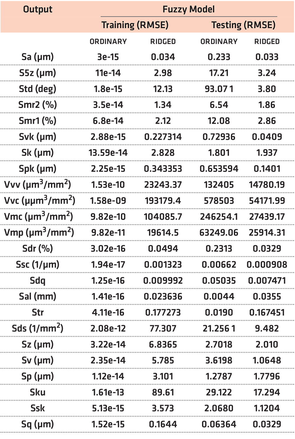
As can be observed from Tables 3 and 4, for the ordinary linear and fuzzy models (without penalizing the weights), the models overfit significantly on the training data set and perform badly on the testing data set across all the 24 areal parameters. The training error is close to zero and this fact is corroborated by Figures 8 and 10. For ridge linear and fuzzy models, the results are better (improved modeling accuracy on the test data). For example, if one considers the Sa para- meter in the two tables mentioned, it can be seen that the training RMSE for both the ordinary linear and fuzzy models are negligible (2e-15 and 3e-15 respectively). The testing performance is respectively 0.531 and 0.233. Although the fuzzy model is better than the lin- ear regression approach (for the ordinary model), there is overfitting on the training data set. The performance is much improved when using the proposed ridge approach. For example, the ridge ordinary fuzzy model has a training RMSE of 0.034 and a testing RMSE of 0.033 (shown in Figure 11). The ridge approach is able to provide a balance in the accuracy of training and testing results.
It should be noted that using the ridge approach on the testing data set, the fuzzy model is able to provide improvement on the modeling accuracy as compared to the linear modeling approach by approximately 75%.
6. Conclusion
This article has presented a new framework based on the ridge Mamdani fuzzy logic system for the mapping of process features to areal surface metrology parameters. The proposed approach represents a non-linear but interpretable solution to the manufacturing informatics modeling problem. The main contribution of this article is the development of a modeling solution that provides consistent accuracy across all the 24 areal parameters on which the results were tested. This is the first time such a framework has been validated across different areal parameters even in the face of a challenging, nonlinear, sparse, multi-dimensional modeling task. In particular, the validation results of the proposed strategy contrast existing areal parameters modeling methods where either results do not generalize across many areal parameters or validation results are difficult to obtain. The proposed approach may benefit from adding an extra layer of inherent in manufacturing systems can be adequately modeled as well as understood. This will be the main focus of future research studies.
Data availability statement
The data that support the findings of this study are available upon reasonable request from the authors.
Ethical Approval
Not Applicable.
Consent to Participate
Not Applicable.
Consent to Publish
Not Applicable.
Authors’ Contributions
Olusayo Obajemu analyzed the datasets and carried out the computer simulation experiments. Moschos Papananias and Thomas E. McLeay designed the laboratory experiments and architected the data acquisition/processing pipeline. Mahdi Mahfouf and Visakan Kadirkamanathan provided technical guidance and validation of the experiments/algorithms developed in the study.
Funding
The authors gratefully acknowledge funding for this research from the UK Engineering and Physical Sciences Research Council (EPSRC) under Grant Reference: EP/P006930/1.
Competing Interests
The authors have no conflicts of interest to declare that are relevant to the content of this article.
Availability of data and materials
Not Applicable.
ORCID iDs
- Moschos Papananias: https://orcid.org/0000-0001- 7121-9681.
- Visakan Kadirkamanathan: https://orcid.org/0000- 0002-4243-2501.
References
- Whitehouse D J 1994 Handbook of Surface Metrology (Boca Raton, FL: CRC Press).
- Jiang X J and Whitehouse D J 2012 Technological shifts in surface metrology CIRP Ann. 61 815–36.
- Mathia T G, Pawlus P and Wieczorowski M 2011 Recent trends in surface metrology Wear 271 494–508.
- Nicola S and Leach R 2018 Information-rich surface metrology Procedia CIRP 75 19–26.
- Grzesik W 2016 Prediction of the functional performance of machined components based on surface topography: State of the art J. Mater. Eng. Perform. 25 4460–8.
- Zhong Z W, Khoo L P and Han S T 2006 Prediction of surface roughness of turned surfaces using neural networks The International Journal of Advanced Manufacturing Technology 28 688–93.
- Grzesik W 2018 Prediction of surface topography in precision hard machining based on modelling of the generation mechanisms resulting from a variable feed rate The International Journal of Advanced Manufacturing Technology 94 4115–23.
- Lu W, Zhang G, Liu X, Zhou L, Chen L and Jiang X 2014 Prediction of surface topography at the end of sliding running- in wear based on areal surface parameters Tribol. Trans. 57 553–60.
- Hu Z-X, Wang Y, Ge M-F and Liu J 2019 Data-driven fault diagnosis method based on compressed sensing and improved multi-scale network IEEE Trans. Ind. Electron. 67 3216–55.
- Neuzil J, Kreibich O and Smid R 2013 A distributed fault detection system based on iwsn for machine condition monitoring IEEE Trans. Ind. Inf. 10 1118–23.
- Dartmann G, Song H and Schmeink A 2019 Big Data Analytics for Cyber-Physical Systems: Machine Learning for The Internet of Things (Amsterdam: Elsevier) (https://doi.org/10.1016/ C2018-0-00208-X).
- Frank A G, Dalenogare L S and Ayala N F 2019 Industry 4.0 technologies: Implementation patterns in manufacturing companies Int. J. Prod. Econ. 210 15–26.
- Sharma A, Kumar S A and Kushvaha V 2020 Effect of aspect ratio on dynamic fracture toughness of particulate polymer composite using artificial neural network Eng. Fract. Mech. 228 106907.
- Worden K, Wieslaw S J and James H J 2011 Natural computing for mechanical systems research: A tutorial overview Mech. Syst. Sig. Process. 25 4–111.
- NFEN ISO. 4287. 1998. Geometrical Product Specifications (GPS). Surface texture: profile method. Terms, definitions and surface texture parameters, 2009.
- Lou M S, Chen J C and Li C M 1998 Surface roughness prediction technique for cnc end-milling Journal of Industrial Technology 15 1–6.
- Segreto T, Karam S and Teti R 2017 Signal processing and pattern recognition for surface roughness assessment in multiple sensor monitoring of robot-assisted polishing The International Journal of Advanced Manufacturing Technology 90 1023–33.
- Plaza E G, López P J N and González E M B 2019 Efficiency of vibration signal feature extraction for surface finish monitoring in cnc machining J. Manuf. Processes 44 145–57.
- Harris P M, Smith I M, Wang C, Giusca C and Leach R K 2012 Software measurement standards for areal surface texture parameters: part 2 comparison of software Meas. Sci. Technol. 23 105009.
- BSEN ISO. 25 178–2: Geometric product specification, surface texture (areal). part 2: Terms, definitions and surface texture parameters. British Standards Institute: London, UK, 2012.
- Löberg J, Mattisson I, Hansson S and Ahlberg E 2010 Characterisation of titanium dental implants i: critical assessment of surface roughness parameters The Open Biomaterials Journal 2 18–35.
- Papananias M, McLeay T E, Mahfouf M and Kadirkamanathan V 2019 A bayesian framework to estimate part quality and associated uncertainties in multistage manufacturing Comput. Ind. 105 35–47.
- ISO 16 610-21. 16 610–21: Geometric product specification (gps)—filtration–part 21: linear profile filters: Gaussian filters. International Standards Organisation, 2011.
- Lotfi A 1965 Fuzzy sets Inf. Control 8 338–53.
- Obajemu O and Mahfouf M 2019 A dirichlet process based type-1 and type-2 fuzzy modelling for systematic confidence bands prediction IEEE Trans. Fuzzy Syst. 27 1853–65.
- Obajemu O, Mahfouf M and Catto J W F 2017 A new fuzzy modeling framework for integrated risk prognosis and therapy of bladder cancer patients IEEE Trans. Fuzzy Syst. 26 1565–77.
- Nabney I 2002 NETLAB: Algorithms for Pattern Recognition (Berlin: Springer).
- Richard L 2013 Characterisation of Areal Surface Texture (Berlin: Springer) (https://doi.org/10.1007/978-3-642-36458-7).
- Xueyi L I, Jialin L I, Yongzhi Q U and David H E 2019 Semi- supervised gear fault diagnosis using raw vibration signal based on deep learning Chin. J. Aeronaut. 33 418–26.
About the authors
Olusayo Obajemu, Mahdi Mahfouf, Moschos Papananias, and Visakan Kadirkamanathan are with the Department of Automatic Control and Systems Engineering, The University of Sheffield, Mappin Street, Sheffield S1 3JD, United Kingdom. Thomas E McLeay is with Sandvik Coromant, Mossvägen 10, Sandviken 811 34, Sweden.
© 2021 The Author(s). Published by IOP Publishing Ltd (https://iopscience.iop.org/article/10.1088/2051-672X/ac28a7). This is an open access article under the CC BY license (http://creativecommons.org/licenses/by/4.0/). It has been edited to conform to the style of Thermal Processing magazine.


 general practice for CQI-9 and AMS2750E")


