


Process control in surface hardening depends greatly on the repeatability of the results. Induction heating facilities stand out in this aspect but challenges arise when it comes to the verification of the expected temperatures. In-situ temperature measurement of a workpiece may be made impossible due to it moving through an enclosed, automated induction facility that lacks built-in sensors. This paper uses transition patterns in the microstructure of the hardened region to reconstruct isothermal contour lines of the temperature field during austenitization. It does so based on a continuous cooling transformation phase diagram and a time-temperature-austenitization diagram of the considered steel. The presented method serves as a practical approach to validate simulations of the inductive austenitizing process and supports simulations of the heat treatment of the work piece. Once these simulations have been iterated upon and validated thoroughly, they may then yield a reconstruction of the entire temperature field during the heat treatment process.
Induction heating techniques have proven a boon to surface hardening, based on their short process times, precise energy input, and resulting low energy usage [1]. The repeatability inherent in electronically controlled induction circuits further lends itself to a high degree of automation within a production chain. Process design for induction hardening, however, is non-trivial as the short heating times allow for little diffusion, giving the microstructure of the base material some influence on the properties of the hardened surface [2]. More difficulties are encountered when defining a new geometry or introducing a workpiece with varying electromagnetic (EM) properties.
In the past, extensive trial and error used up valuable machine time to find new process parameters. Nowadays, simulation techniques such as the Finite Element Method (FEM) take on much of the burden by predicting the distribution of heat generation during the heat treatment and inform design decisions before the first test run is scheduled [3-5]. In general, several simplifications and assumptions are always made when simulating a problem (not least of which are estimates of unknowns, such as surface emissivity or heat-transfer coefficients), and any simulation needs to be verified in order to produce meaningful data [6,7].
The most direct way to verify process simulations is to compare the resulting temperature field with data obtained from experiments [7-9]. Temperature data in particular is relatively easy to obtain [10] — as opposed to the magnetic field distribution within steel parts — and is not contingent on further material models, as the phase or stress distributions are. The concrete difficulty of obtaining the temperature data for a given process can vary wildly from one facility to another. Many modern industrial heat-treatment facilities are sealed off from any outside interference, simultaneously increasing the controllability of the process and decreasing the risk of injury due to interaction with moving, conducting, and/or hot parts [11]. These safety and control features come at the expense of accessibility, hindering measurements if no instrumentation has been included during the construction of the facility or the design of the process control software.
Ideally, the heat-treatment process is monitored, so that temperature at a certain heating stage or the time dependent temperature of each workpiece is logged, stored, and transferable for quality control and simulations. Often, however, this is not the case. On top of that, if the heat-treatment process also involves moving workpieces or induction coils, they may obscure line of sight for ad-hoc pyrometer measurements and make instrumentation of samples impossible.
The method described in this article deals with such a case, where there was virtually no temperature data available. This was due to the induction facility being highly automated (and therefore enclosed), but not instrumented. While material data could be gained from treated and untreated workpieces, there was no information available on the heat-treatment curve the bearing underwent during the process, and recording one was infeasible.
The only data point was an estimate of 1,050°C, obtained through glimpsing into the induction oven from the intake conveyor and seeing a bright yellow shine through the rotating heating assembly. Needless to say, that one temperature value of such questionable origin could hardly be used to verify the rather complex multi-physics simulation that would have to be implemented further in the future.
While there was no way of measuring the temperature in-situ, the temperature history of the hardened workpiece still left its traces in its microstructure. This paper aims at describing a method of combining metallurgical data from phase diagrams usually available to the heat-treatment facility with a micrograph analysis of a surface hardened sample in order to deduce several depths of different transition temperatures within the material. Consequently, a general numerical temperature distribution fitted to these temperature-depth pairs can be used to verify the estimated surface temperature.
Experimental characterization
Phase diagram
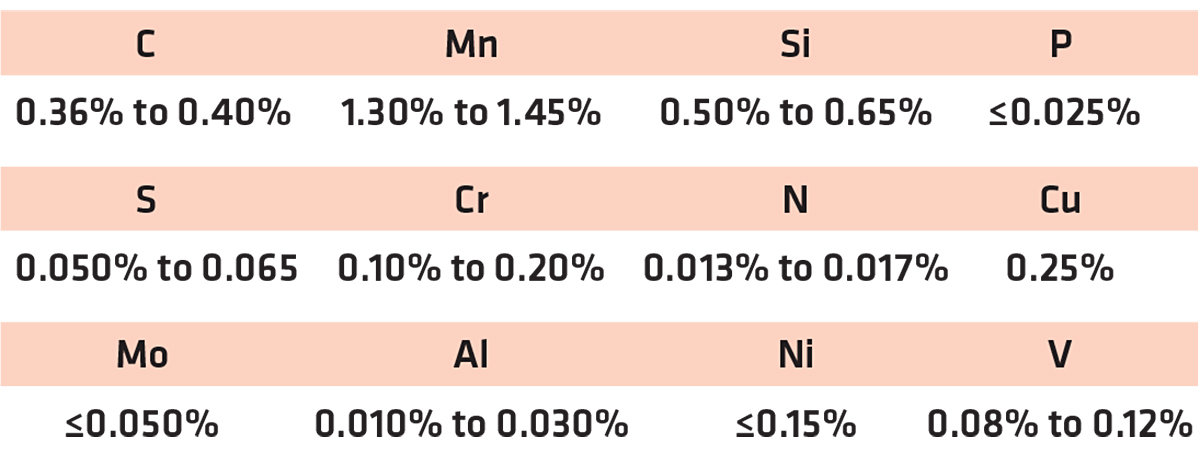
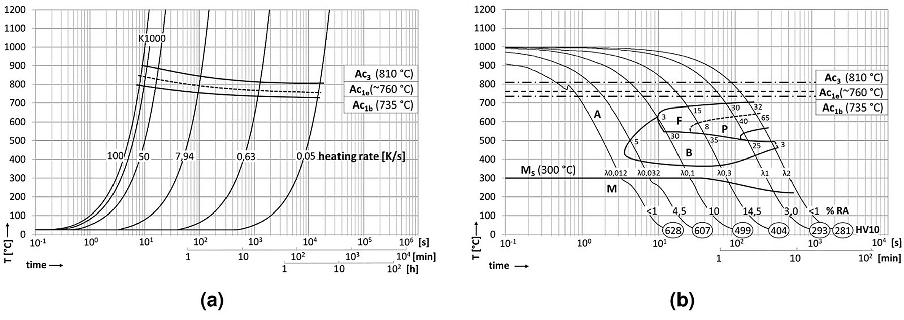
The steel in this study was a modified C38 tempering steel forged into shape and subsequently inductively surface hardened. Its chemical composition is specified by the manufacturer to be according to the ranges listed in Table 1. Its base microstructure was pearlitic-ferritic with a grain size of approximately 30 μm and contained randomly distributed MnS inclusions. These did not affect the hardening process and are irrelevant to the following investigation. The hardening was performed to heat treat a minimum depth of 3mm from the surface. Samples for dilatometry were cut from untreated zones of the component shafts, measuring 10mm in length and 4mm in diameter and tested using a Bähr DIL805A quenching dilatometer. The phase transformation temperatures were determined at a heating rate (HR) of 3 Kmin-1, noting a distinct split of Ac1 into a starting temperature Ac1b and an end temperature Ac1e. All of these temperatures increase with heating rate, so that the heat treatment in practice, with a heating rate of 81.67 Ks-1, experiences Ac1b at 790°C, Ac1e at 840°C and Ac3 at 895°C. Differing cooling rates were examined at this heating rate up to an austenitization temperature of 1,000°C, with 10 seconds of holding time to allow for appropriate austenitization of the samples. The material exhibits a distinct bainite nose between λ0.02 and λ0.1. Figure 1 shows the time-temperature-austenitization (TTA) and continuous-cooling-transformation (CCT) diagrams generated from these experiments.
Micrographs
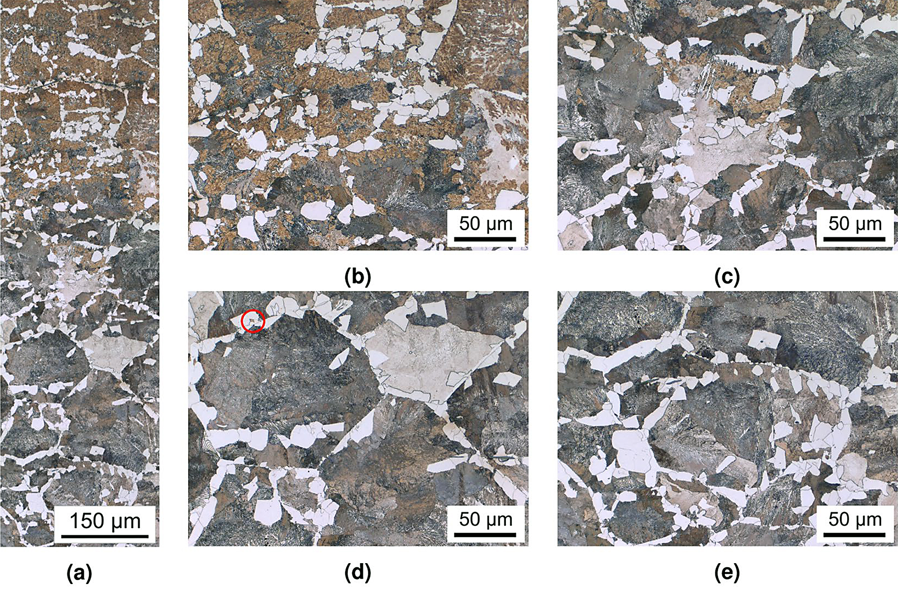
The heat-treated part consists of a bearing journal surface surrounded by flanges. The shaft was cut through the bearing’s axis, and one journal surface was trimmed to fit into the bedding. The sample was ground and polished with a 1 μm diamond suspension as the finishing step, and subsequently etched using a 3% nitric acid solution, with the prepared sample shown in Figure 2 as an overview.
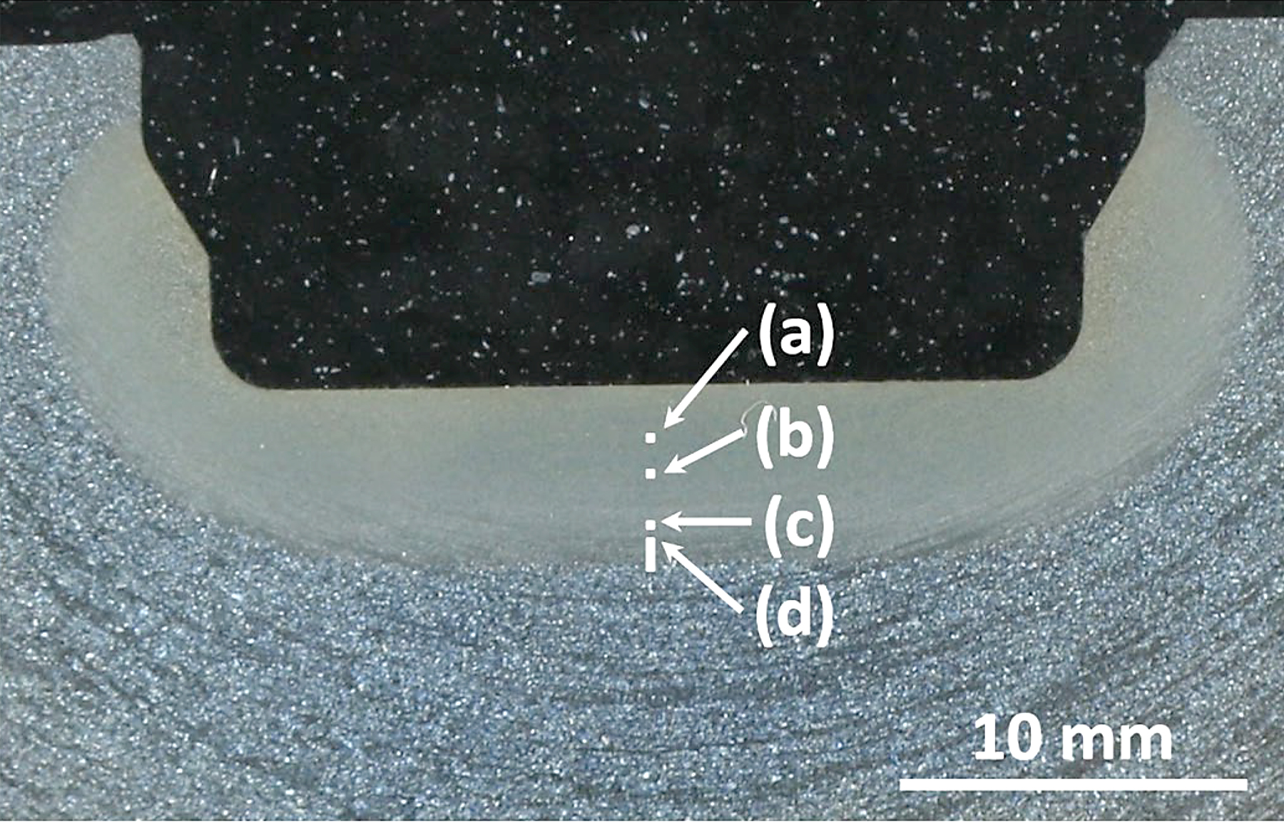
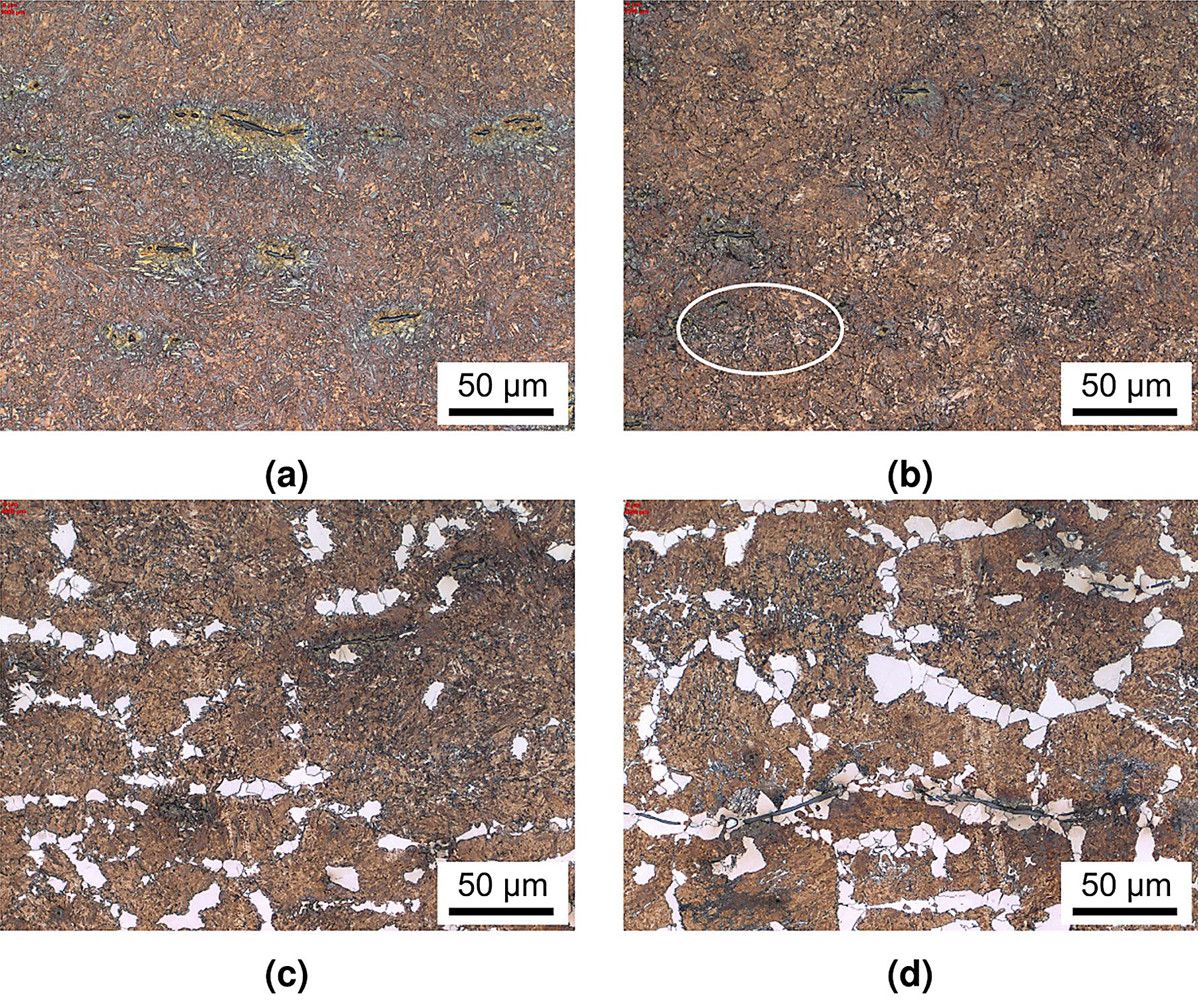
This and all following micrographs were taken by using a Zeiss Axio Imager M2m optical light microscope with an AxioCam MRc5 installed. The diameter of the bearing is 50mm while the hardened zone of the material extends to about 5 mm depth at the journal centerline. The surface is austenitized within 12 s and quenched to room temperature within another 10 s, roughly following the λ0.012 line in Figure 1a. The expected microstructure within the hardened zone is therefore purely martensitic. Figure 2 describes the positions of the following micrographs, with Figure 2a through 2c and the upper part of 2d being represented in Figure 3, and the entirety of 2d shown in Figure 4.
Hardness gradient
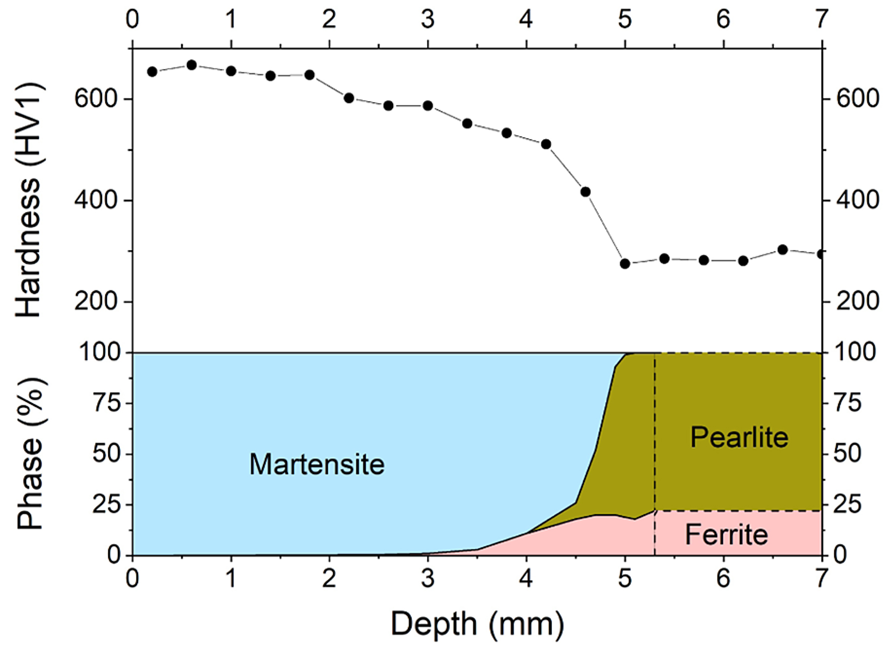
A line of Vickers hardness measurements was taken along the same centerline as the micrographs, using a Qness Q10A+ Vickers hardness tester. A measuring load of 1 kgf (HV1) was set to allow for close placement of indentations. Figure 5 shows the hardness as a function of depth projected over a phase fraction analysis that was performed on the micrographs shown in Figures 3 and 4. The hardness gradient is an amalgamation of not only the phase transition, but other influences such as grain size and phase structure. While discerning the exact influences of each effect would go beyond the scope of this report, the hardness is representative of the continuously varying microstructure in the hardened zone. This variation is due to the transformation from ferrite-pearlite to austenite (and later, during quenching, to martensite) by the heat input of the temperature field during the performed inductive surface hardening. Thus, the plateau at the end of the hardness gradient corroborates the depth of the Ac1b temperature determined through micrograph analysis.
Reconstruction of the temperature field
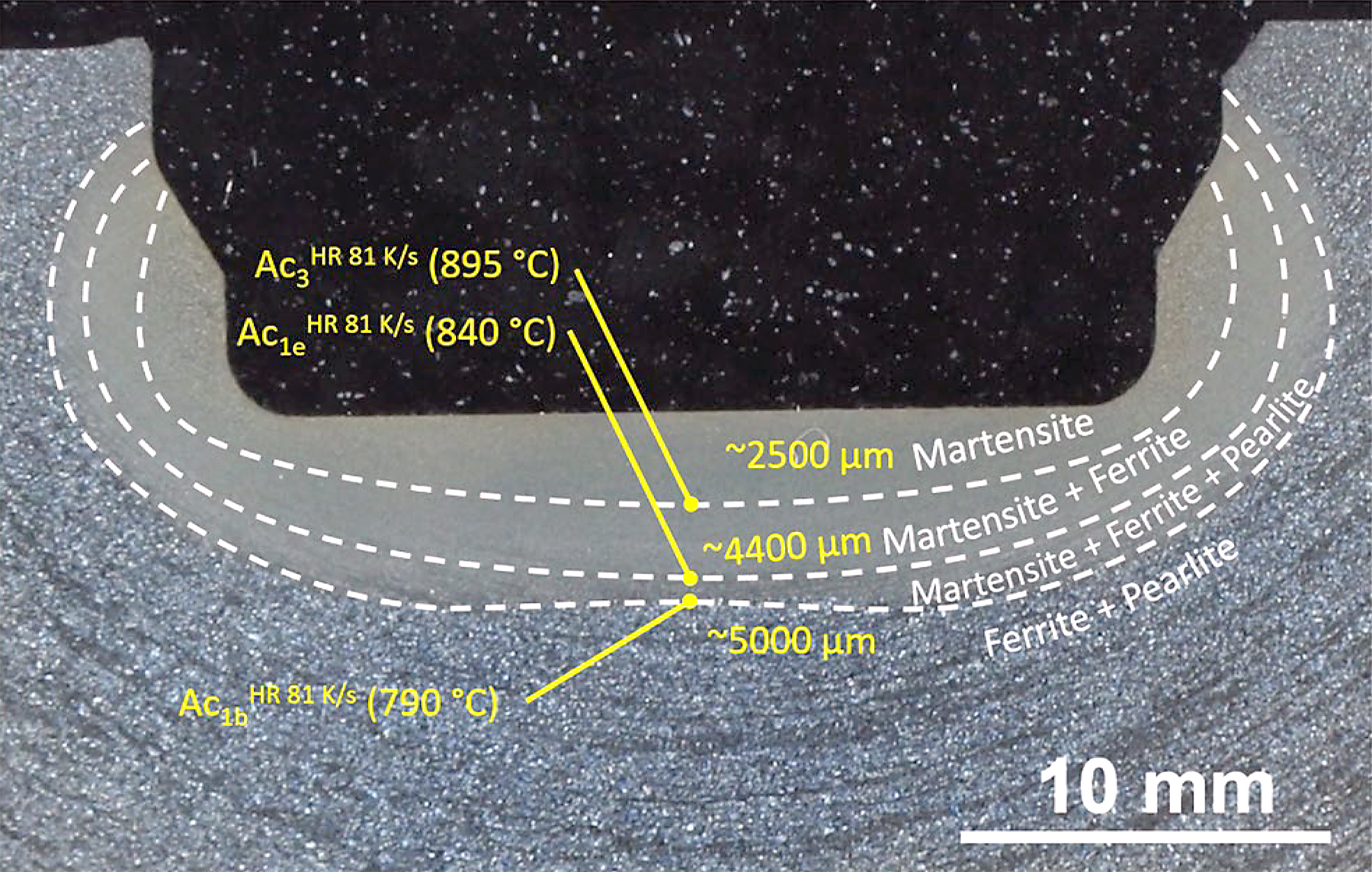
The silhouette of the thermal gradient that the material experienced during heat treatment can be guessed from the overview in Figure 2. However, the detailed analysis in Figures 3 and 4 reveals the transition zones at which the material crossed the transition temperatures depending on the fast austenitizing and short holding time depicted in Figure 1a. The transformation temperatures Ac3, Ac1e and Ac1b are determined at the depths of 2,500 μm, 4,400 μm and 5,000 μm, respectively. The performed hardness measurement corroborates these depths fairly well with average hardness of 650HV1 at the surface coinciding with the predicted 628HV10 of the quenched martensite described in Figure 1b until a depth of about 2,000 μm. While they were attained with a differing load on the Vickers indenter, the resulting hardness values can be assumed to be comparable, as the indentation size effect only starts taking effect at the micro scale (100 gf indentation load) [12]. The subsequent hardness drop can be attributed to the incomplete dissolution of ferrite, which has not completely transformed into the austenitic phase during the heating process, as seen in Figures 3b-d and 5. An even steeper drop toward the base hardness begins below 4,200 μm and corresponds to further increasing amounts of ferrite and the beginning appearance of pearlite (see Figures 4b,c and 5), indicating the temperature during austenitization only slightly exceeding Ac1b and thus starting the pearlite to austenite transformation but not completing it.
The precise depths can be incorporated into the overview image to show an approximation of the transformation zones present during the heat treatment, as depicted in Figure 6.
The temperature at the surface may still be of interest, since it is the control parameter of choice in most automated induction facilities. Analytical solutions describing the temperature distribution of induction heated cylindrical parts exist [13] but ignore the cooling of the surface.
A simplified, axisymmetric cylindrical model of the bearing was calculated by FEM simulation with load parameters approximating those of the industrial heat treatment, with detailed parameters given in Table 2 and Figure 7. The model uses fixed time increments of 250 ms to leapfrog between a linear harmonic solution to the electromagnetic problem and a heat transfer solution that uses heat sources obtained from the previous EM calculation, which provides the temperature distribution for the next EM step. This interaction is regulated by a python script controlling the ABAQUS software used to calculate the results.
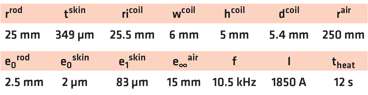
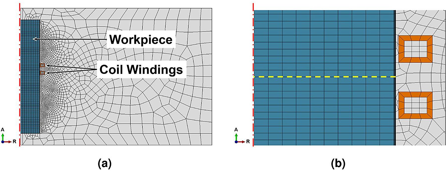
The 5° slice of rod had a radius of rrod = 5 mm and length of lrod = 150 mm. A complex claw-shaped inductor of proprietary geometry encompassed ≈150° of the bearing, which rotated constantly at a distance of 0.5 mm during the hardening process.
Since the simplified model was only an axisymmetric slice of the whole circumference, the inductor was represented as a coil of rectangular cross section (wcoil = 6 mm wide by hcoil = 5 mm tall) with two turns dcoil = 5.4 mm apart, distanced 0.5 mm from the bearing surface. The model air space had a radius of rair = 250 mm. Homogeneous Dirichlet boundary conditions were defined at all surfaces; these confined the magnetic field to the simulated geometry by acting as magnetic insulation. This was well suited since the field was assumed to be axisymmetric and to not extend past the dimensions of the defined cylinder of air. The mesh within the rod was generated from hexagons with a set width of e0rod = 2.5 mm. The skin depth was 349 μm and divided into 15 elements geometrically scaled from e0skin = 2 μm at the surface to e1skin = 83 μm. The air mesh was generated procedurally to scale from 1.5mm at the coil surface to e∞air = 15mm at the model boundary, while the coils were modeled one element thick with a wall thickness of 1mm. The load was a sine wave current with an amplitude of I = 1,850 A and a frequency of f = 10.5 kHz. This amperage was based on a measurement on the induction coil but increased slightly to result in a solution close to the assumed maximum surface temperature of 1,050°C. The heat-transfer model used only the mesh of the rod and applied a convective film boundary condition of hair = 20 Wm-2K and ambient radiation condition assuming the surface emissivity to be ε = 0.7. The initial temperature distribution was set to be a uniform room temperature 25°C, and the rod was heated for theat = 12 s.
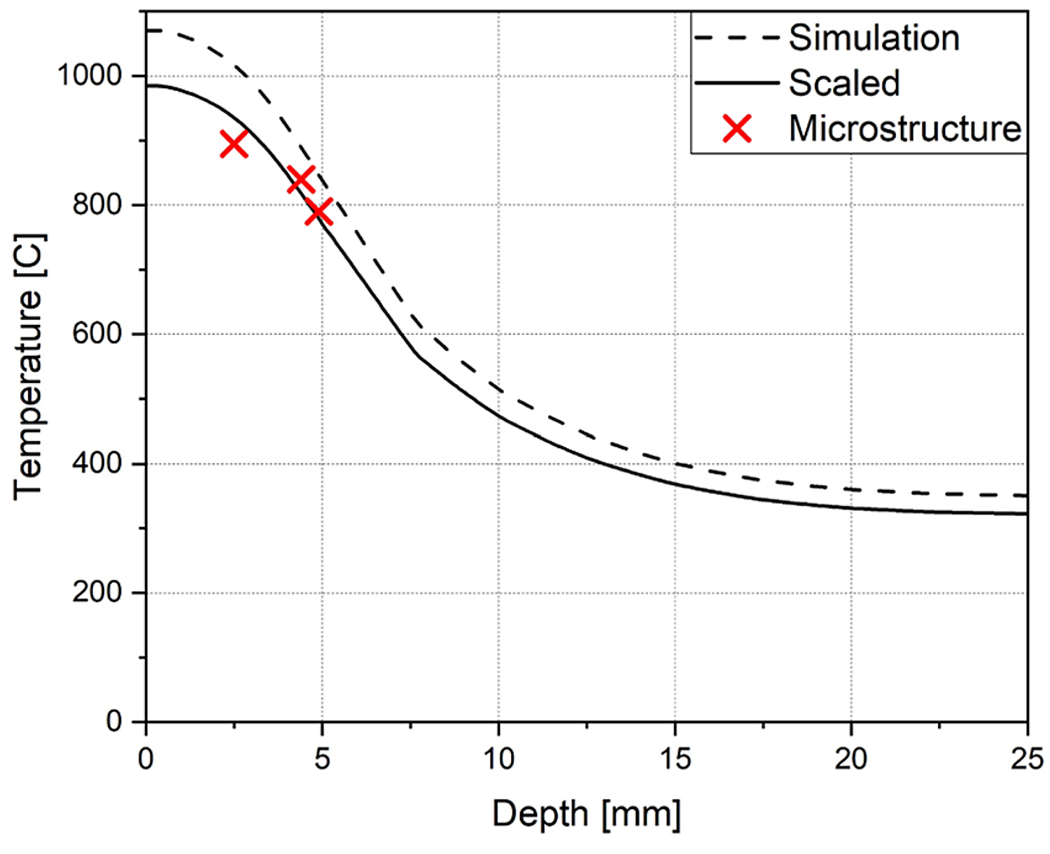
The resulting distribution shows the temperature envelope, i.e. the maximum reached throughout the process, along the path shown in Figure 7b. While the surface temperature was dialed in to the assumed 1,050°C, its envelope was found to be too high for the observed internal transformation depths. Assuming a linear scaling of the entire distribution, it was fitted to the measured depth of phase transitions and their associated temperatures, minimizing the sum of squared residuals. This resulted in an estimated surface temperature of 985°C (see Figure 8).
Discussion
As stated in the introduction, the presented method represents an approach for obtaining temperature data of a surface hardening heat-treatment process where there is no in-situ measurement possible or available. The thorough investigation of the microstructure in the surface-hardened region supplies rather precise ranges of the transition from one microstructural region to another. It is important to note the transitions are not sharp but rather transitional areas due to local differences in chemistry because of production related segregations and possible variations in the temperature distribution imposed by the inductive heat generation. However, the evaluated transition depths in combination with a TTA-recording for the process conditions supply the transition temperatures for the considered heat treatment quite precisely on a macro scale.
The actual transition temperatures in the bearing journal may be somewhat higher, since the TTA-information is drawn from tiny samples with a diameter of 4mm that experience homogeneous heating in the dilatometer compared to the 50mm diameter of the bearing, where a certain degree of overheating is necessary since its core acts as a heat sink during the heating process.
While the transition lines shown in Figure 6 are based entirely on the evaluation of the microstructure of the central line of the bearing and a qualitative assessment of the overview image, it is of course possible, though work intensive, to generate an arbitrarily fine grid on the etched area, detailing the exact shape of the zones. For verifying a simulation of the heat-treatment process, however, a handful of temperatures at different known points is usually sufficient.
The FEM simulation used to extrapolate the surface temperature serves as an example for the verification process: It is a preliminary study using a simplified geometry with estimated process parameters and a linear electromagnetic material model. While the surface temperature fitted in Figure 8 is close to the expected 1,050°C, the simulation is still in need of calibration and with depth, temperature drops faster than expected. The phase transition regions determined in the microstructure indicate a slower drop of the temperature, which the electromagnetic model needs to be adjusted to account for.
Further steps in the modeling procedure now include updating the model geometry, parameters, and material model to closer match the physical bearing and result in a better fit with the temperature distribution observed in Figure 6.
Conclusions
The following conclusions can be drawn from this work:
- The temperature history at given points on or slightly below the surface of a surface-hardened part can be reconstructed based on microstructural features found by a post-mortem microscopy study provided that a time-temperature austenitization diagram of the material, which has been recorded for process relevant cooling rates, is available.
- FEM simulations of the thermal problem can be validated by comparing the calculated temperature field with those reconstructed temperatures. Unknown simulation parameters such as surface-to-air heat transfer coefficients can inversely be determined by an iterative approach.
References
- Rudnev, V., Loveless, D., Cook, R. & Black, M. Handbook of induction heating, 1st edn (CRC Press, New York, NY, USA, 2017).
- Eggbauer, A. et al. In situ analysis of the effect of high heating rates and initial microstructure on the formation and homogeneity of austenite. Journal of materials science 54, 9197–9212 (2019).
- Boadi, A., Tsuchida, Y., Todaka, T. & Enokizono, M. Designing of suitable construction of high-frequency induction heating coil by using finite-element method. IEEE Transactions on Magnetics 41, 4048–4050 (2005).
- Sun, J., Li, S., Qiu, C. & Peng, Y. Numerical and experimental investigation of induction heating process of heavy cylinder. Applied Thermal Engineering 134, 341–352 (2018).
- Istardi, D. & Triwinarko, A. Induction heating process design using comsol multiphysics software. Telkomnika 9, 327–334 (2011).
- Mevec, D., Raninger, P., Prevedel, P., Jászfi, V. & Antretter, T. Getting to know your own induction furnace: Basic principles to guarantee meaningful simulations. HTM Journal of Heat Treatment and Materials 74, 267–276 (2019).
- Vieweg, A. et al. Experimental and numerical analysis of the inductive tempering of a qt-steel. HTM Journal of Heat Treatment and Materials 72, 199–204 (2017).
- Di Luozzo, N., Fontana, M. & Arcondo, B. Modelling of induction heating of carbon steel tubes: Mathematical analysis, numerical simulation and validation. Journal of Alloys and Compounds 536, 564–568 (2012).
- Sadeghipour, K., Dopkin, J. & Li, K. A computer aided finite element/experimental analysis of induction heating process of steel. Computers in Industry 28, 195–205 (1996).
- Kranjc, M., Zupanic, A., Miklavcic, D. & Jarn, T. Numerical analysis and thermographic investigation of indction heating. International Journal of Heat and Mass Transfer 53, 3585–3591 (2010).
- Nacke, B. & Baake, E. (eds.) Induction Heating: Heating | Hardening | Annealing | Brazing | Welding (Vulkan Verlag, 2016).
- Broitman, E. Indentation hardness measurements at macro-, micro-, and nanoscale: a critical overview. Tribology Letters 65, 23 (2017).
- Carslaw, H. S. & Jaeger, J. C. Conduction of heat in solids, 2nd edn (Oxford: Clarendon Press, 1959).
Acknowledgements
This topic originally featured at the ECHT 2019 – European Conference on Heat Treatment – Bardolino (Italy), 5–7 June 2019. The authors gratefully acknowledge the financial support under the scope of the COMET program within the K2 Center “Integrated Computational Material, Process and Product Engineering (IC-MPPE)” (Project No 859480). This program is supported by the Austrian Federal Ministries for Transport, Innovation and Technology (BMVIT) and for Digital and Economic Affairs (BMDW), represented by the Austrian research funding association (FFG), and the federal states of Styria, Upper Austria and Tyrol.
Author contributions
Writing — Original Draft and Presentation: D.G.M.; Writing — Review and Editing: D.G.M., P.R., and P.P.; Conceptualization: D.G.M., P.R., P.P., and V.J.; Investigation: P.P. lead, V.J. supporting; Resources: P.P.; Methodology: D.G.M., P.R., and P.P.; Supervision, Project Administration, and Funding Acquisition: P.R.
Competing interests
The authors declare no competing interests.
© The Author(s) 2020; www.nature.com/articles/s41598-020-63328-6
This article is an open access article distributed under the terms and conditions of the Creative Commons Attribution (CC BY) license (http://creativecommons.org/licenses/by/4.0/). This article has been edited to conform to the style of Thermal Processing magazine.


 general practice for CQI-9 and AMS2750E")


