


You are probably somewhat familiar with the thermocouple, or you wouldn’t be reading this article. But there are important points about thermocouples that must be understood and that will help you to make an informed selection between sensor types and avoid potential problems in your application.
First, we need to clear up a common misconception about how thermocouples work. You may have been told something like “a thermocouple produces a small voltage created by the junction of two dissimilar metals.” This simplification of the thermocouple is at best only half true and very misleading. The reality is that it is the temperature difference between one end of a conductor and the other end that produces the small electromotive force (emf), or charge imbalance, that leads us to the temperature difference across the conductor.
OK, simple enough, but how do you actually measure this emf in order to discern its relationship to temperature?
The “emf” or electromotive force refers to a propensity level, or potential for current flow as a result of the charge separation in the conductor. We refer to this propensity for current flow between two points as its potential difference, and we measure this difference of potential in volts. But in order to actually measure the emf or voltage difference, we need two points of contact. That is, we must complete the circuit by adding a return electrical path. If we simply choose to use the same metal as a return path, the temperature difference between the ends of your original conductor would simply create an equal and opposite EMF in the return path that would result in a net EMF of zero — not very useful for measuring temperature. This relationship is expressed by the “Law of Homogeneous Material” as follows (see Wikipedia.org):
 A thermoelectric current cannot be sustained in a circuit composed of a single homogeneous material by the application of heat alone, and regardless of how the material may vary in cross-section. That is, temperature changes in the wiring between input and output will not affect the output voltage, provided all wires are made of the same material as the thermocouple. No current flows in the circuit made of a single metal by the application of heat alone.
Different conductive metals will produce different levels of emf or charge separation relative to the thermal gradient across the metal. Thomas Seebeck discovered this principle in 1822 and it is known today as the “Seebeck Effect.” Thus, we can apply the “Seebeck Effect” and make it useful for measuring temperature by using a different metal for our return path, and then relating the differences in charge separation between the two metals to the temperature between the ends. We join these metals at the start of our return path by forming a junction between them — that is, the junction simply joins our circuit and is not the source of the emf, as is often inferred by the traditional definition of a thermocouple.
Now, at the other end of our closed thermocouple circuit, we can measure a voltage between the two wires that will be proportional to the temperature between the ends. By the Law of Homogeneous Materials expressed earlier, the thermocouple wires can each pass into and out of cold areas along their path without the measuring instrument detecting the temperature changes along the path because the emf created as the continuous wire enters and leaves an area will sum to zero and have no net effect on our final measurement.
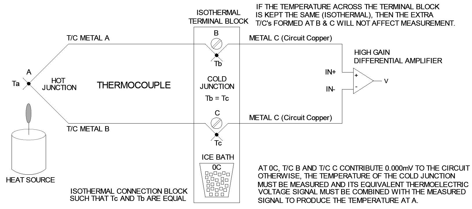
We still have a conceptual problem though — how do we measure the voltage at the open end of our thermocouple without introducing additional “thermocouple” voltages into our measurement system? That is, the connection points of the T/C to the measurement system (which is typically copper) will itself act as a thermocouple. It turns out that the effect of these additional thermocouples on our measurement system can be minimized by simply making sure the connections are at the same temperature. This principle is expressed by “The Law of Intermediate Materials” as follows (see Wikipedia.org):
The algebraic sum of the thermoelectric emfs in a circuit composed of any number of dissimilar materials is zero if all of the junctions (normally at the cold junction) are maintained at a uniform temperature. Thus, if a third metal is inserted in either or both wires while making our cold junction connections, then as long as the two new junctions are at the same temperature, there will be no net voltage contribution generated by the new metal in our measurement system.
So, our ability to overlook these unintended thermocouples in our measurement will depend on how well we can maintain both cold junction connections at the same temperature. This is often easier said than done, and small thermal gradients will usually occur, often as a result of the self-heating of components across the circuit board. Other thermal gradients can be driven by heat generated from adjacent circuits, nearby power supplies, or via variable wind currents or cooling fans in the system. For any thermocouple transmitter, special care must be taken to minimize these sources of error.
A third law for thermocouples that helps us combine emfs algebraically is “The Law of Successive or Intermediate Temperatures” stated as follows (see Wikipedia.org):
If two dissimilar homogeneous materials produce thermal emf1 when the junctions are at T1 and T2, and produce thermal emf2 when the junctions are at T2 and T3, then the emf generated when the junctions are at T1 and T3 will be emf1 + emf2, provided T1<T2<T3.
Still, our measurement of the open-end voltage across our thermocouple only relates the thermoelectric voltage to the difference in temperature between both ends. That is, we need to know the temperature of the cold junction at one end in order to extract the sensed temperature from the other end (hot junction). Ideally, if both connections made at the measuring end were at 0°C, their thermoelectric equivalent voltage contributions to our measurement would be 0mV, and we could easily determine the sensed temperature directly from our measured voltage. Since this can’t be easily assured, the actual temperature of the cold junction connection point is usually measured separately. Then the measured T/C signal can be compensated for the thermoelectric contribution of the connection point or “cold junction,” and we can extract the actual temperature of the remote end of our thermocouple by a mathematical combination of either the measured temperature or its thermoelectric equivalent voltage. See Figure 1.
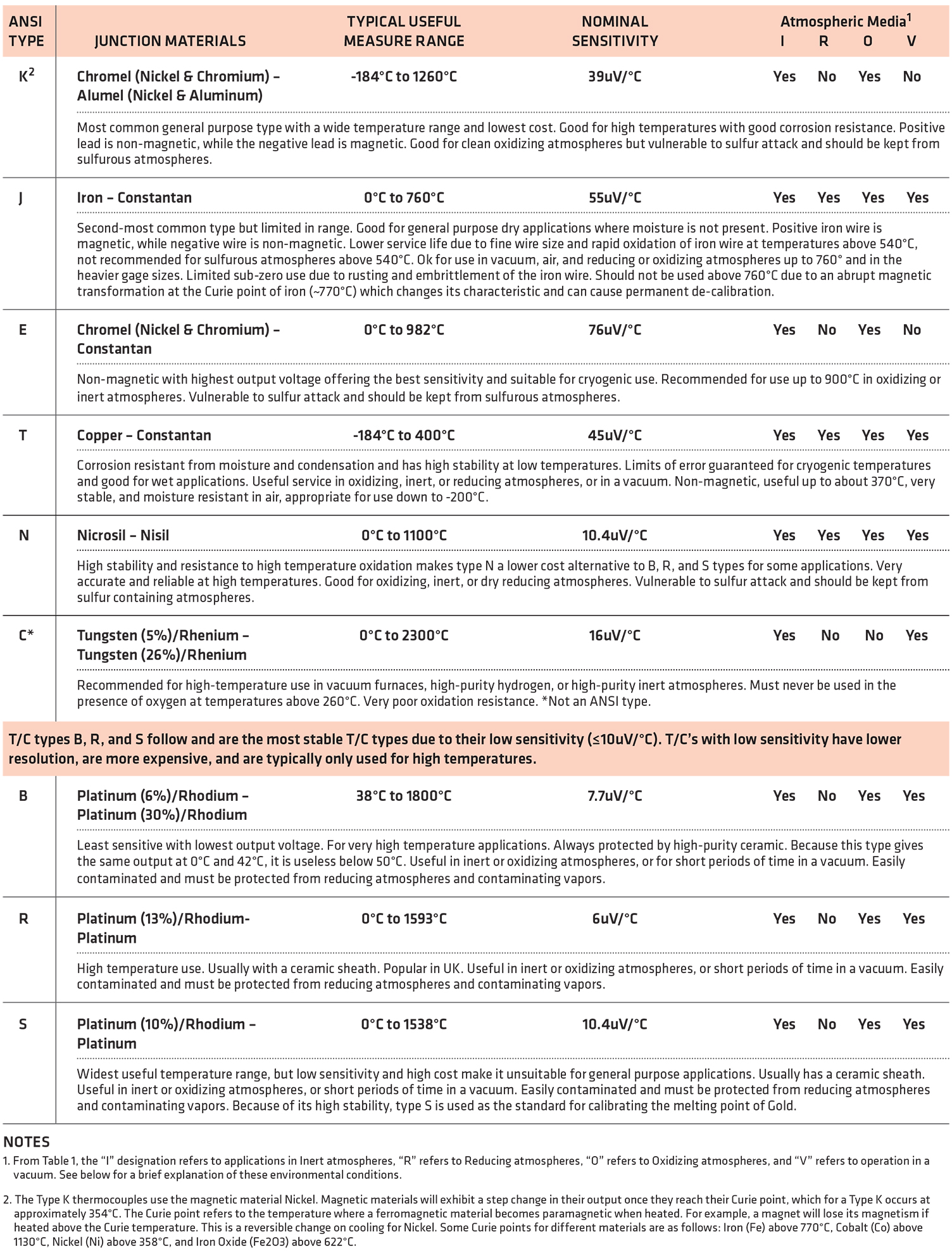
Although we could form a thermocouple by joining any two dissimilar conductors, a number of standard thermocouple types are available that use specific metals combined to produce larger predictable output voltages with respect to their thermal gradients. The most common types are listed in Table 1.
Notes (Table 1)
• 1. From Table 1, the “I” designation refers to applications in Inert atmospheres, “R” refers to Reducing atmospheres, “O” refers to Oxidizing atmospheres, and “V” refers to operation in a vacuum.
• 2. The Type K thermocouples use the magnetic material nickel. Magnetic materials will exhibit a step change in their output once they reach their Curie point, which for a Type K occurs at approximately 354°C. The Curie point refers to the temperature where a ferromagnetic material becomes paramagnetic when heated. For example, a magnet will lose its magnetism if heated above the Curie temperature. This is a reversible change on cooling for Nickel. Some Curie points for different materials are as follows: iron (Fe) above 770°C, cobalt (Co) above 1,130°C, nickel (Ni) above 358°C, and iron oxide (Fe2O3) above 622°C.
From Table 1, we see that the selection of a specific T/C type will be guided by the useful measurement range of the sensor, its sensitivity, its material, and its operating environment. Sensor cost may also play a role in this decision as certain types are more expensive than others — for example, the platinum-based sensor types are generally more expensive by virtue of their platinum content.
Because materials used at extreme temperatures can be permanently altered by their application environment, you must also consider the atmospheric conditions of their application as noted in Table 1.
An “inert atmosphere” refers to an environment of a gaseous mixture that contains little or no oxygen and primarily consists of non-reactive gases or gases that have a high threshold before they react. Nitrogen, argon, helium, and carbon dioxide are common components of inert gas mixtures.
A reducing or “reduction atmosphere” refers to an environment in which oxidation is prevented by the removal of oxygen and other oxidizing gases or vapors. This usually refers to environments containing nitrogen or hydrogen gas. For example, it is often imposed in annealing ovens to relax metal stresses and prevent metal corrosion.
Nitrogen is also used in some electronic soldering ovens to improve the performance and/or appearance of the solder joint.
An “oxidizing atmosphere” is a gaseous environment in which the oxidation of solids readily occurs due to the presence of excess oxygen. Contrast this to the reducing atmosphere described earlier in which the available oxygen is reduced or eliminated. Many combustion processes will use oxidizing atmospheres. Many substances oxidize rapidly when heated sufficiently in the presence of free oxygen. The oxidation that results refers to the transformation that occurs when portions of compounds and molecules break free from the material allowing the free oxygen to attach to the remaining material and form oxides. For example, it is commonly used inside kilns for firing pottery in order to drive materials to convert to their oxide forms, or to control material color. When copper carbonate is fired, the carbon detaches and burns off as the copper-carbon bond is broken, the available oxygen rushes in to attach to the copper, forming a copper oxide.
A “vacuum atmosphere” refers to an environment or volume of space that has been evacuated of free matter, such that its gaseous pressure is much less than the surrounding atmospheric pressure. Note that a perfect vacuum is not practically achievable as atoms and particles are always present in the atmosphere, but the quality of a vacuum environment would refer to how well it approaches a perfect vacuum, as indicated by how low its environmental pressure is relative to atmospheric pressure.
The maximum temperatures of any thermocouple type are generally limited by the type of insulation used.
Points of Consideration When Using Thermocouples to Measure Temperature
Since accuracy will ultimately play a significant role in selecting a sensor type, we should be familiar with potential sources of error when making temperature measurements with thermocouples. Some of these considerations may steer us from one T/C type to another, or perhaps to another sensor type, like RTD for example.
T/C Sensor Inaccuracy
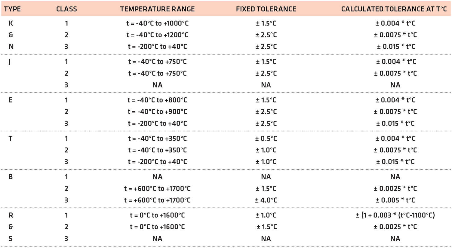
Some manufacturers of thermocouple sensors may have their own accuracy designations different from the standard designation described in Table 2, and those should always be consulted first, as they sometimes offer better than standard performance. But by the IEC 584-2 standard, thermocouple sensors are divided into three accuracy classes: Class 1, Class 2, and Class 3. By this standard, two tolerance values apply for a given temperature and thermocouple type: a fixed value and a calculated value based on the sensor temperature. The larger of these two values is normally taken as the sensor tolerance (note that Type C has been excluded below as it is not an ANSI type designation).
T/C Sensor Non-Linearity
The non-linearity of the thermocouple output itself can vary up to several percent or more over the full temperature range of a T/C type. The mathematical relationship between sensor temperature and output voltage is modeled via a complex polynomial to the 5th through 9th order depending on the T/C type. Some transmitters will take special measures to adjust their output response for these non-linearities and make their outputs linear with the input temperature range. Other applications are not concerned with linearizing the transmitter’s output response relative to the sensor temperature, and their response will instead be linear with the thermoelectric voltage signal of the sensor. In many cases, a given thermocouple will be nearly linear over a smaller range of its application temperature, and some non-linearity will be acceptable without applying special linearizing methods.
Likewise, some low-cost transmitters will use analog methods to shift the output to adjust for this non-linearity, and this generally works best over smaller or truncated portions of the sensor range. Some modern digital instruments will actually store thermoelectric breakpoint tables in memory to accomplish multi-segment linearization of a T/C range and return the corresponding temperature for a given voltage measurement.
Depending on your application, the lack of linearization can be a significant source of error if you fail to account for it.
T/C Sensor Sensitivity
As mentioned earlier, we noted that any conductor subject to a thermal gradient along a dimension will generate a voltage difference along that same path, and this is known as the Seebeck effect. Different materials will exhibit different magnitudes of thermal emf related to the difference in temperature. Combining two different materials and joining them at one end allows us to complete a circuit, build the thermocouple, and actually measure the relative voltage. The relative sensitivity of the thermocouple refers to its Seebeck coefficient, which is simply a measure of its incremental change in thermocouple voltage corresponding to an incremental change in temperature (i.e. dV/dT in mV/°C or uV/°C). This is essentially the slope of the thermocouple function (voltage versus temperature) at a selected temperature. It’s important to note that just as a thermocouple varies its linearity over temperature, its relative sensitivity is also temperature dependent. That is, some thermocouples will be more or less sensitive for smaller portions of their application temperature range. Table 1 gave a nominal sensitivity figure for the thermocouple over its entire application range to help differentiate the thermocouples by sensitivity, but over smaller ranges, this figure can vary considerably. T/Cs that have lower sensitivity will have lower resolution. These are generally used at higher temperatures where the need to resolve a given temperature to a high degree of accuracy is not a requirement. Likewise, if you need to resolve temperature to a fraction of a degree, you would select a T/C with higher sensitivity and a corresponding higher resolution.
Sensor Drift, Aging, and De-Calibration
Drift or de-calibration of a thermocouple sensor refers to the process in which the metallurgy of the thermocouple wire has been altered as a result of its exposure to temperature extremes, usually for prolonged periods of time. It may also occur inadvertently by failing to consider the “entire” operating range of a sensor application including its over-range and under-range or fault conditions. Drift usually occurs as a result of the diffusion of atmospheric particles into the metal at extreme temperatures. But it can also occur due to the diffusion of impurities and chemicals from a thermocouple’s insulation or protective sheath into the T/C wire at temperature extremes. It is always good policy to check the specifications of the thermocouple or probe insulation, as it usually limits the effective operating ambient of the thermocouple itself.
Choice of Extension Wire
For thermocouples that must pass over a long distance, thermocouple extension cable is often used. Extension cables are generally used to lower the total cost of the sensor and will use similar materials to the thermocouple itself or materials better suited for the intervening environment. The important thing to remember about the use of an extension cable is that its thermoelectric behavior sometimes only approximates that of the thermocouple, and it will usually limit the applicable range of the thermocouple by virtue of its insulation. Be cognizant of the extension wire used in an application and its limitations, as it can be an increasing source of error if applied improperly with respect to temperature and environment. Note that for base metal thermocouples (J, K, N, E, and T), the extension wire conductor is the same composition as the corresponding thermocouple and will exhibit the same thermoelectric properties as the thermocouple itself. However, for noble metal thermocouples (R, S, and B), the wire is usually a different alloy that will only approximate the noble metal thermoelectric properties but over a more limited range.
The conductor material is different because the noble metals contain platinum, which would be very expensive to use as extension wire. Use of a different material is often not a problem, as these T/C types are generally used at higher temperatures and have a lower resolution, such that the small error contribution of using a different but similar extension wire is less significant. In all cases, the maximum application temperature will be limited by the type of insulation used by the extension wire and this is an important factor in selecting the proper extension wire for a given application.
Response Time
The response time refers to the time interval between the application of a sudden change in temperature to a sensor and its corresponding change in output. This change is frequently defined as the time it takes for the sensor to reach 63.2 percent of its final value. A rapid response time or shorter time constant helps to reduce error in systems that encounter rapid changes in temperature. It is dependent on several parameters, such as T/C dimensions (wire size), construction, tip configuration, and the medium to which it makes contact. For example, if a thermocouple penetrates a medium with high thermal capacity and rapid heat transfer, the effective response time would approach that of the thermocouple itself (its intrinsic response time). But if the thermal properties of the medium are poor, still air for example, the response time can be 100 times greater. For an insulated or ungrounded thermocouple, response time can vary from a fraction of a second (small diameter) to several seconds (large diameter). For non-insulated or grounded thermocouples, the typical time varies from a small fraction of a second (small diameter) to a few seconds (large diameter). In general, thermocouple temperature sensors have the fastest response times, especially when compared to RTD sensors. It is generally their small point of contact and low thermal mass that gives them a faster response time. But similar to an RTD, the response time of a thermocouple measurement will also depend on its insulation. That is, you can specify a grounded (non-insulated) or ungrounded (insulated) thermocouple. A grounded thermocouple junction puts the material junction in direct contact with the surrounding case metal, which gives it a faster response time. But the grounded tip is also more prone to noise pickup and may increase measurement error, in particular when wired to non-isolated measuring instruments. You should tend to use an ungrounded (insulated) sensor to avoid these issues, but only when sensor isolation and response time are not over-riding issues for your application. If your application absolutely requires a fast response time, you will probably need a grounded tip and will have to take other measures to combat noise pickup or isolate your signal, such as selecting a compatible isolated transmitter.
Cold Junction Compensation
Near room temperature, the major source of error for any thermocouple sensor is that which is attributed to cold junction compensation (CJC). Because thermocouples only measure the difference in temperature between two points and not the absolute temperature of the sensor, we must apply cold junction compensation (also reference junction compensation) in order to directly relate the measured voltage to the sensor temperature. Realistically, our temperature measurement can only be as accurate as our method of cold junction compensation. This compensation contributes significant error to our measurement and, in order to minimize cold junction error, the measurement cold junction circuit has to accomplish two things very well:
The connection points to the thermocouple must be kept at the same temperature, or “isothermal.” Any temperature gradient from one point to the other will be a source of error (Recall the Law of Intermediate Materials explored earlier).
The actual temperature of the connection points must be measured accurately, or at least as accurately as the thermocouple itself. The response time of the CJC sensor can also be a factor in maintaining accuracy, in particular for systems that require a fast response time but may have unstable cold-junction ambient.
While our thermocouple allows us to make precise differential temperature measurements, we need to make sure that the pair of terminals that connect to the T/C and comprise our cold junction are at the same temperature or “isothermal” with one another. Not doing so would introduce an errant T/C voltage into our measurement. We also have to make sure that the cold junction has enough thermal mass so that it will not change temperature over the time it takes for us take the two measurements necessary to convert the T/C signal into the actual temperature at the remote end.
Connection Problems
Potential measurement error is often a result of poor connections, which drive unintended thermoelectric voltage contributions to our measurement voltage. If you need to increase the length of thermocouple wires, you must use the correct type of T/C extension cable for the thermocouple. Substitution of any other type will add errant thermocouple junctions to our measurement system. If terminals are used to connect the wires, then you must additionally select connectors made up of the same material type, unless you can ensure that the connections are kept at the same temperature. You also need to observe the proper polarity when making connections.
Other connection problems arise when an incompatible material type is used for a given environment, or where extension wire has been mismatched to the sensor or its environment. For example, thermocouples that use iron as a material will be subject to corrosion that may impede continuity, particularly in wet environments.
Thermal Shunting and Immersion Error
All thermocouples have some mass, and heating this mass will absorb some energy that will ultimately affect the temperature you are trying to measure. In some applications, the T/C wire will act like a heat-sink at the point of measurement, and that can result in significant measurement error. The use of thin T/C wires helps minimize this effect in many applications. For example, consider a thermocouple immersed in a small vial of liquid to monitor its temperature. Heat energy may travel up the T/C wire and dissipate to the atmosphere reducing the temperature of the liquid around the wires. Or, if the thermocouple is not sufficiently inserted into the liquid, the cooler ambient air surrounding the wires may actually conduct along the wire and cool the junction to a different temperature than the liquid itself. The use of thinner wires would cause a steeper thermal gradient along the wire at the junction between the ambient air and the liquid itself. However, thin wires have a higher resistance, and this can drive other errors. It may be better to use shorter thin T/C wires connected to much thicker thermocouple extension wires in order to alleviate the resistance effect for some applications.
Lead Resistance
To minimize the effects of thermal shunting and to improve response time, thin T/C wire is generally used. The use of thin wire is also at least partially driven by the type of wire that is more expensive, in particular for the platinum-based, noble metal types R, S, and B. But the downside to using thin wire in some systems is that it increases the sensor resistance making it more sensitive to noise, and potential IR errors driven by the measuring instrument. Care should be taken to ensure that the loop resistance of a wired thermocouple be kept low, and a general rule of thumb is to keep it below 350Ω to avoid excess error and below 100Ω would be better.
Noise
The thermocouple output voltage is a small signal that is prone to errant noise pickup. Likewise, the fine leads are made from other materials than copper and have a higher resistance, making them more sensitive to noise pickup, in particular AC-coupled noise. Further, the high gain that generally operates on these small signals further amplifies this noise. Other sources of thermal noise result from unstable ambient temperatures at the cold junction. The generally fast response time of the thermocouple exhibits this noise at the output as the cold junction generally tracks the junction temperature much slower than the T/C sensor itself, usually as a result of its larger thermal mass and the sensor used to measure its temperature. Noise can usually be minimized by twisting the wires together to make sure that both leads pick up the same signal (i.e. common mode noise is rejected).
Likewise, minimize the length or loop area where the cables part to make a connection to the instrument. Route T/C wires defensively, keeping them from combining with power wires. Operation in noisy environments or nearby electric motors may benefit from the use of screened extension cable. If noise pickup is suspected, simply switch off suspect equipment and observe if the reading changes.
Common-Mode Voltage
Although the thermocouple signals are small, much larger voltages may exist at the instrument itself due to the presence of common-mode voltages driven by inductive pickup along the sensor wire or via multiple earth-ground connections in the system. Inductive pickup is commonly a problem when using a thermocouple to sense the temperature of a motor winding or power transformer. Multiple earth grounds may be inadvertent, perhaps when using a non-insulated or grounded thermocouple to measure the temperature of a hot water pipe. In this instance, any poor connections to earth ground may drive a few volts of difference between the pipe and measuring instrument. The use of high-quality, high-gain, differential instrument amplifiers will generally reject this noise as it is common to both input leads, but only as long as the voltages remain within the common-mode input range of the instrument amplifier (usually limited to ±3V to ±5V by the internal DC voltage rail of the instrument). As noted with errant noise earlier, it usually helps to twist the wires together to make sure that both leads pick up the same signal (i.e. common mode noise is rejected by the amplifier). Also keep the length short or the loop area small where the cable conductors part to make a connection to the instrument.
By now you should realize that choosing a temperature sensor for an application is not as simple as picking a thermocouple type with a compatible temperature range. You must consider the sensor material type, the application temperature range, the relative sensitivity of the sensor, the limitations of its insulation material, and its reaction with the measurement environment. You must also be aware of the inherent limitations of the thermocouple and potential error sources in its application.


 general practice for CQI-9 and AMS2750E")


