


In this column, we will discuss the determination of the quench factor as it is used in quench factor analysis. This will lead into a discussion of determining the time-temperature-property (TTP) curve to be used in quench factor analysis.
Introduction
The quench factor, τ, is defined as:
 where τ is the quench factor, t is the time (sec), and Ct is the critical time. The collection of the Ct points, also known as the C-curve, is like the time-temperature-transformation curve for continuous cooling.
In general, the Ct function is described as [1]:
 where Ct is the critical time required to precipitate a constant amount of solute. The meaning of each of the constants are described in the previous article.
To determine the parameters K1, K2, K3, K4, and K5, it is first necessary to have the C-curve. C-curve data is scarce, and of limited availability. Some coefficients for the Ct function are shown in the previous column and in [2]. Once the C-curve, or time-temperature-property curve, is obtained, the values of the coefficient are obtained by repeated iterations (and minimum error) until the best fit to the C-curve is achieved [3].
One of the problems with the equation for the C-curve is its complex nature and dependence on K2–K5. Different sets of K2–K5 can provide similar fits to the data, with similar errors, but can provide wildly different time-temperature-property curves [4]. Fitting the time-temperature-property coefficients is severely non-linear, and results in errors regardless of the method used. Independent physical data offer much better fits to the data and result in reduced errors in the C-curve. Data such as the solvus temperature (K4), solute diffusivities (K5) and enthalpy for precipitation (K7) substantially reduce the fitting errors and non-linearity and offer physical meaning to the data and fit. Use of many data points (> 10) reduces the errors. Combining interrupted quench data and continuous cooling data is very effective in reducing C-curve errors.
One additional source of error is some aluminum alloys have competing precipitates forming during quenching and aging. For instance, many types of precipitates may be observed in a single sample. The precipitates may be at the grain interior or at the grain boundary. There may be different precipitates present (θ and S). They could also be different coherency (incoherent and semi-coherent). This results in multiple C-curves, like the pearlite and bainite curves in time-temperature-transformation diagrams for steels. Quench factor analysis, as created by Evancho and Staley [3], assumes only one primary precipitate.
Determination of Property Data as a Function of Quench Rate
From the previous discussion, the modeling of aluminum alloys is dependent on the data generated through interrupted quench data or from continuous cooling data. Typically, it is necessary to measure the quench path of several sheets of material, and then measure the properties after processing. The quench factor is determined for each quench path and associated with the measured properties. Typically, hardness and tensile properties have been used.
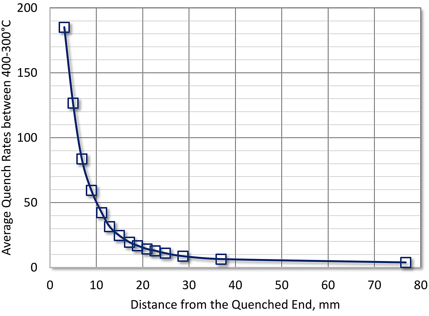
The Jominy end quench [5] provides a method of determining both the quench factor and the C-curve. The Jominy end-quench test has many advantages for determining quench sensitivity of aluminum and other alloys such as titanium [6]. The method offers many advantages over traditional quenching of sheet and plate. The observed quench rates vary from 200°C/s at 3 mm from the quenched end to less than 3°C/s at 78 mm from the quenched end [7] (Figure 1). Further, it is a data-rich specimen. Once quenched, and hardness and conductivity has been measured, the specimen can be sliced at specific locations for TEM and DSC analysis [8] [9].
Properties are then related to the quench factor by the equation:
 where p is the property of interest, pmax is the maximum property attainable with infinite quench rate, and K1 is -0.005013 (natural log of 0.995).
By rearranging the above equation, the quench factor, Q, can be determined for hardness on the Jominy end quench:
 where HVN is the hardness at a specific location on the Jominy end quench bar, and Hmax is the maximum hardness. The maximum hardness, Hmax, is generally an average of the first several hardness indentations.
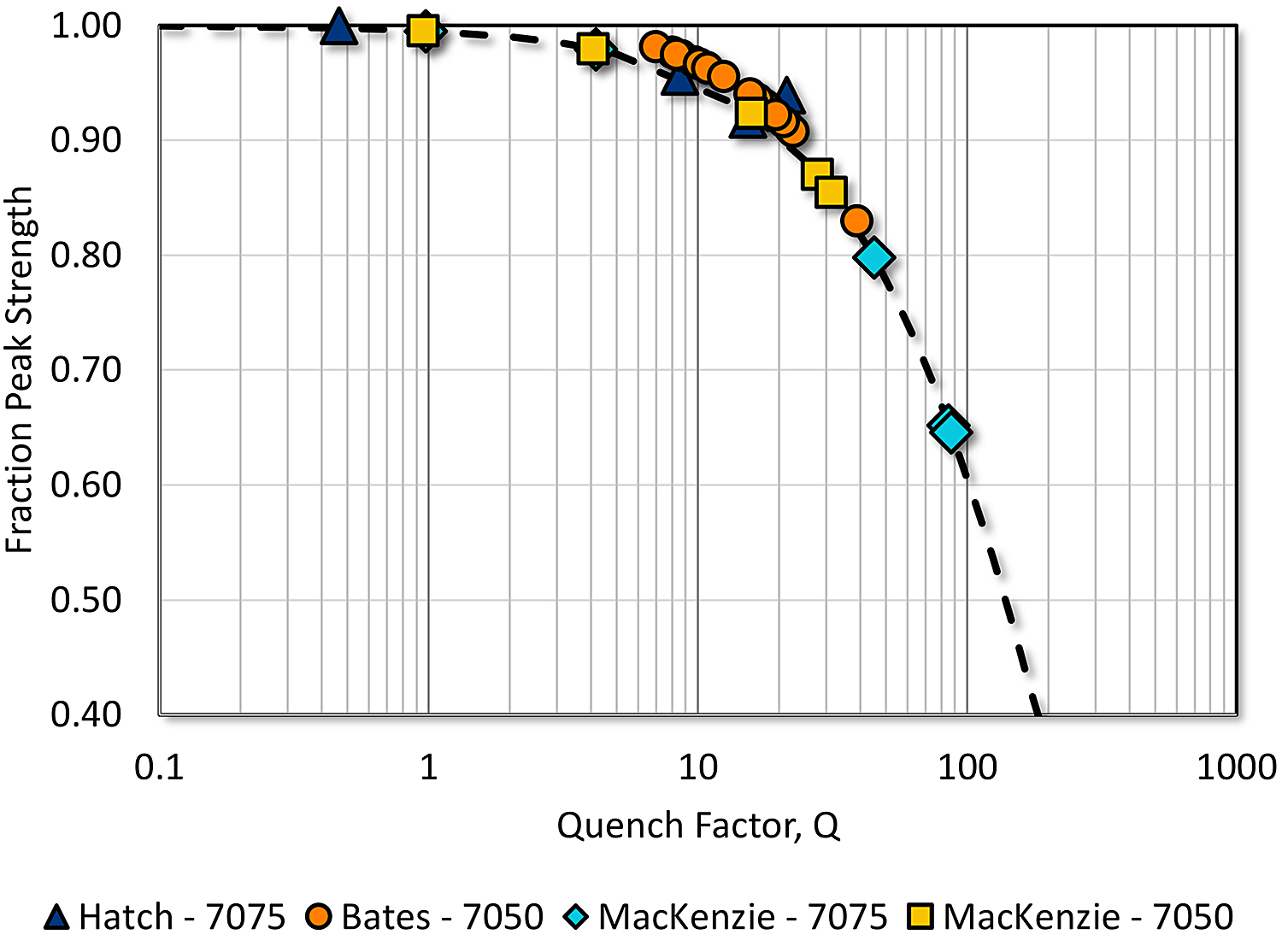
Therefore, for a specific set of processing conditions, the quench factor can be determined for multiple quench rates, using the Jominy end quench. The data generated can be used to predict properties occurring in similar material and similar operating conditions. This is illustrated in Figure 2. In this figure, the percentage of the attainable property from hardness (7075-T6 and 7050-T6 from the Jominy end quench), is compared with that obtained by Hatch [10] by quenching individual panels and measuring the yield strength. This method allows for the determination of the quench factor without knowledge of the C-curve.
Conclusion
In this short column, we have illustrated methods of determining the quench factor as a function of quench rate. In the next column, we will discuss a method of determining the C-curve, and the different coefficients in the C-curve equation.
Should you have any questions regarding this article, or have suggestions for any additional columns, please contact the writer or the editor.
References
- J. T. Staley, “Quench Factor Analysis of Aluminum Alloys,” Mat. Sci. Tech., vol. 3, p. 923, November 1987.
- D. S. MacKenzie, “Metallurgy of Heat Treatable Aluminum Alloys,” in Heat Treating of Nonferrous Alloys, vol. 4E, G. E. Totten and D. S. MacKenzie, Eds., Materials Park, OH: ASM International, 2016, p. Metals Handbook 2A.
- J. W. Evancho and J. T. Staley, “Kinetics of Precipitation in Aluminum Alloys During Continuous Cooling,” Met. Trans., vol. 5, pp. 43-47, January 1974.
- R. T. Shuey, M. Tiryakioglu and K. B. Lippert, “Mathematical Pitfalls in Modeling Quench Sensitivity of Aluminum Alloys,” in Proc. 1st Intl. Sym. Metallurgical Modeling for Aluminum Alloys, 13-15 Oct. 2003, Pittsburgh, PA, 2003.
- J. E. Jominy, “Standardization of Hardenability Tests,” Metals Progress, vol. 40, pp. 911-914, December 1941.
- J. W. Newkirk and D. S. MacKenzie, “The Jominy End Quench For Light-Weight Alloy Development,” Journal of Mat. Eng. Perf., vol. 9, no. 4, pp. 408-415, August 2000.
- D. A. Tanner and J. S. Robinson, “Effect of Precipitation During Quenching On The Mechanical Properties Of Aluminum Alloy 7010 in the W-temper,” J. Mat. Processing, vol. 153, no. 11, pp. 998-1004, 2004.
- D. S. MacKenzie, “Effect of Quench Rate on the PFZ Width in 7XXX Aluminum Alloys,” in Proceedings from 1st International Symposium on Metallurgical Modeling for Aluminum Alloys, 13-15 October, 2003, Pittsburgh, PA, 2003.
- D. S. MacKenzie, Quench Rate and Aging Effects in Al-Zn-Mg-Cu Aluminum Alloys, Rolla, MO: University of Missouri — Rolla, 2000.
- J. E. Hatch, Aluminum: Properties and Physical Metallurgy, Metals Park, OH: American Society for Metals, 1984.
- W. L. Fink and L. A. Wiley, “Quenching of 75S Aluminum Alloy,” Trans. AIME, vol. 175, p. 414, 1948.
- C. E. Bates, “Quench Factor-Strength Relationships in 7075-T73 Aluminum,” in Proc. Int. Conf. on Long-Term Storage Stabilities of Liquid Fuels, San Antonio, TX, 28 July – 01 August 1986.
- M. Avrami, “Kinetics of Phase Change I,” J. Chem. Phys., vol. 7, pp. 1103-1112, February 1939.
- M. Avrami, “Kinetics of Phase Change II,” J. Chem. Phys., vol. 8, pp. 212-224, February 1940.
- G. P. Dolan, R. J. Flynn, D. A. Tanner and J. S. Robinson, “Quench factor analysis of aluminum alloys using the Jominy End Quench technique,” J. Mat. Sci. Tech., vol. 21, no. 6, pp. 687-692, 2005.


 general practice for CQI-9 and AMS2750E")
 steels")


