


Often, the terms “digital twins” or ICME (Integrated Computer Materials Engineering) are used when talking about computer modeling of actual parts or the behavior of materials in industry. There exists a big push to collect as much data as possible and convert these data to computer models that accurately predict the process parts go through from billet to final product. All this collection of data begs the question: “How can all these data be used?” In heat treatment modeling, there exists a need to accurately represent the boundary conditions of the furnaces and quenching systems used. High thermal gradients that exist in heat treatment have a significant effect on phase transformation timing, the overall strain in the part, and the in-process and residual stresses. Lab tests with carefully controlled environments and probes are great for base data that can be used in general cases, but the experimental conditions in the lab rarely correlate to commercial furnaces or quench systems running real parts. Thus, the use of thermocouples, embedded in actual parts, and data collection systems have become the gold standard in data collection for heat treatment.
For this article, time-temperature data from a salt bath heating and high-speed water quench process will be examined. A utility tool originally developed internally at DANTE Solutions and now available to the public, called HTCFit, is used to determine the Heat Transfer Coefficient (HTC) that the part surface experiences during heating and quenching. HTCFit uses a forward finite-element (FE) method to quickly execute a series of FE models, having different heat transfer boundary conditions based on the input parameters, to find the best fit to the time-temperature data using an optimization function. This forward method is preferred because it can capture the effects of latent heat due to phase transformations and capture the different thermal properties of individual phases.
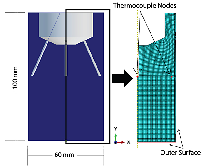
The quench probe for this experiment was a cylinder made of AISI 304 stainless steel, with a 60 mm diameter and a 100 mm height, as shown schematically in Figure 1. A 50 mm threaded hole, 25 mm deep, was countersunk in the top of the cylinder, and from there five holes were drilled to insert thermocouples. One thermocouple was placed on the centerline of the cylinder, representing the core, and four thermocouples spaced radially from the center to measure the temperature near the surface. The top of the probe was sealed with a 50 mm NPT threaded cap and rod to allow an egress for the thermocouple leads. The experiment was performed by submersing the probe in a bath of molten salt at 870°C until fully soaked.
Then, the probe was quickly transferred to a highly agitated water bath where it was quenched to room temperature. The time-temperature data for heating was collected every second while the quench data was collected every 30 milliseconds to capture the rapid quench. Data from the core thermocouple and one near-surface thermocouple were used to fit the surface convection coefficient experienced by the probe for the heating and quenching process. A complication was discovered when viewing the collected data and the probe after the experiments. Some molten salt had entered the cap and housing, causing a slight ripple in the core thermocouple data between 700°C and 800°C. Despite this anomaly, the HTCFit algorithm could ignore this noise and the fit was largely unaffected. Often, when dealing with raw data there is some level of cleanup that is required before processing. Other than separating these data into heating and quenching, no other data cleanup modifications were required.
With the experiments performed and the data collected, an FEA model of the probe is constructed. An axisymmetric CAD model was created and meshed with 3,217 nodes and 3,075 elements, with finer elements near the surfaces to capture the steep thermal gradients present during heating and quenching, as shown in to Figure 1. Nodes, correlating to the positions of the thermocouples on the actual probe, and the outer surfaces were named and defined in the FEA model. The model information was passed to DANTE Solutions’ MatSim software, along with the time-temperature data, the initial guess for the HTC values, and an HTC range to search. For this exercise, the HTC is fit by part surface temperature because the probe is being quenched with water. HTC vs time can also be fit for processes such as gas-quenching, where the HTC and ambient quenchant temperature can vary with time. The heat-up fitting took three minutes to process six design variables while running 77 FEA simulations. The quenching fitting took 2.5 minutes to process seven design variables while running only 40 FEA simulations, despite having significantly more time-temperature data, due to the frequency at which quench data were saved: 6,419 data pairs for the quench vs. 699 pairs for heating.
Results
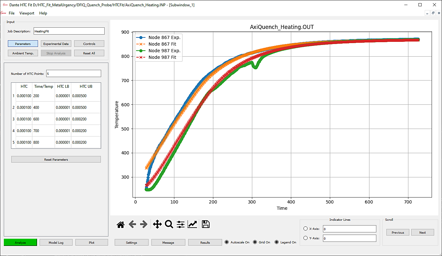
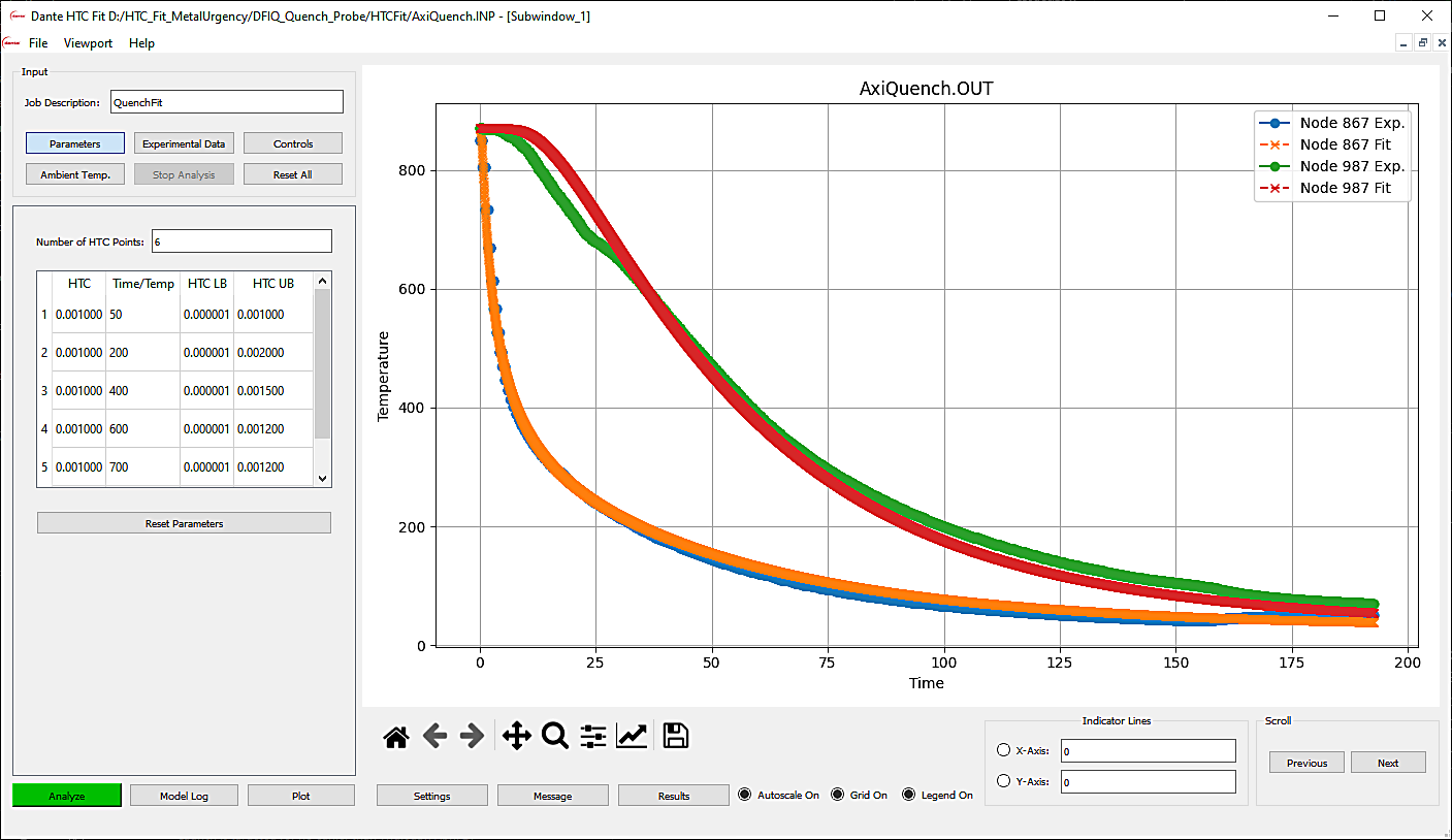
Results for fitting are shown in Figures 2 and 3. The heating and quenching fit is good overall. The near-surface fit, shown in blue and orange, is the best fit of the two data sets. The core fitting, shown in green and red, is off in the higher temperature range where the salt entered the probe housing and skewed the data, but otherwise the predicted core temperature follows the heating and cooling data trend reasonably.
The HTC results from HTCFit, shown in Figure 4, reveal that the expected vapor blanket stage, typical of water and oil quenches, is absent for the high-speed water quench. The high agitation quickly removes heated water and replaces it with fresh quenchant so no stable vapor blanket forms. The peak value determined by HTCFit was 15,700W/(m2*°C). This value dipped slightly early in the quench until the surface dropped below 400°C, where the HTC value drops off as convection forces take over in the quench tank.
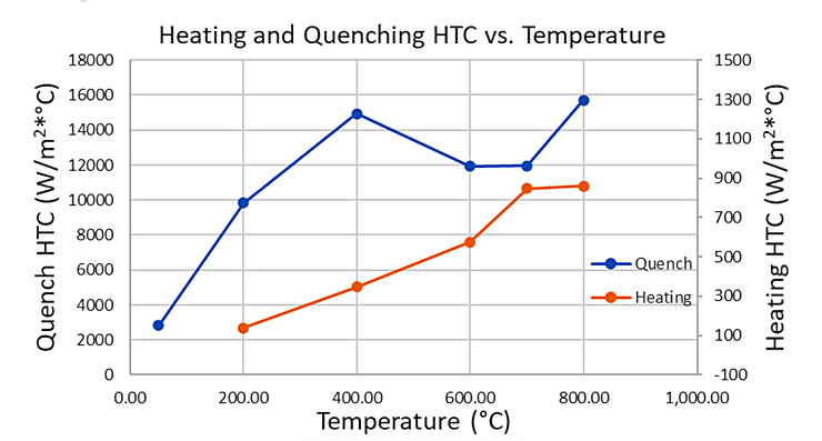
The HTC value was found to be 140W/(m2*°C) at the start of heating and steadily increased to a final value of 860W/(m2*°C) at higher temperatures. The HTC for the salt bath increased almost linearly as the part heated until about 600°C, when radiation begins to play its part in the heat transfer.
Conclusion
The need to process time-temperature data into useful heat transfer coefficients for modeling has been fulfilled using HTCFit. The quench probe designed for this application successfully captured the rapid temperature changes present during heating and quenching. The process of determining relevant HTC values is not limited to this probe, or to this particular heating and quench process, and is robust enough to handle virtually any part geometry and quenchant where time-temperature data is collected with embedded thermocouples. The derived heat transfer coefficients can now be used in finite element simulations to accurately simulate the convection boundary conditions present during the heat treatment process. Accurately representing the boundary conditions leads to more accurate models, especially where stress and strain are considered, providing an accurate “digital twin,” and shedding light on the black box that is heat treatment.


 general practice for CQI-9 and AMS2750E")


