


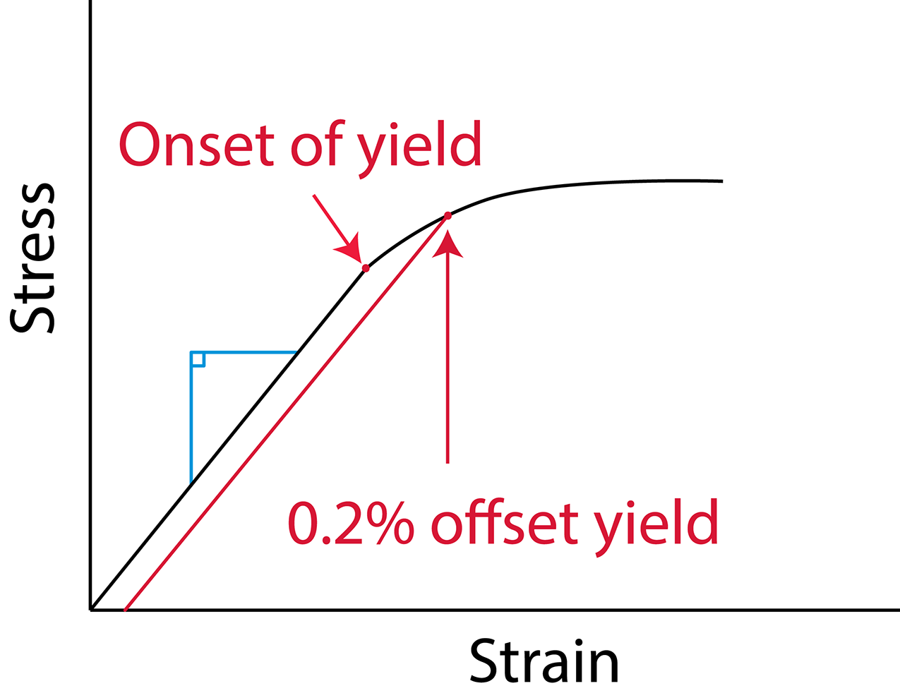
Understanding the plastic behavior of steel plays a crucial role in manufacturing. From raw billet to parts in service, some form of plastic deformation can be found in every step of the manufacturing process, heat treatment not excluded. In fact, I used to joke in Materials and Manufacturing Process class that you should include the words “plastic deformation” in every answer to get full credit. On a macro scale, plastic deformation is simply any permanent shape change to the part. Microstructurally, deformations take the form of atomistic dislocations and planes of slip in the matrix of the base material. Engineers understand plasticity with the classic stress/strain plot from a tension or compression test, Figure 1.
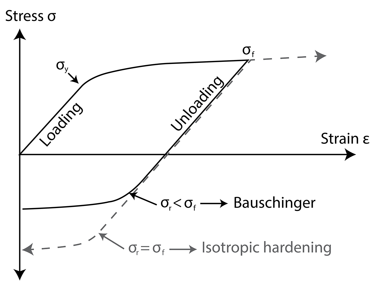
When a tensile sample is pulled in the testing equipment, the resulting strain imparts a stress in the sample. This stress initially increases in a linear relationship to the imparted strain, and the slope of this line, stress over strain ratio, is called Young’s Modulus. If the load is released in this region, the elastic range, the sample will return to its original shape, largely unaffected. If the sample continues to be pulled, the stress increases until the sample begins to yield, or plastically deform. The onset of yield is sometimes not as obvious in some materials, so engineers developed the 0.2% offset yield strength, which ensures that the entire macroscopic cross section is yielding, and not just individual regions.
A well-studied phenomenon, called the Bauschinger effect, named after German engineer Johann Bauschinger, states that after a material plastically deforms in one direction, it will be easier to deform in the opposite direction. As an example, tubular steel products are mechanically tested in the hoop direction, and this curvature is often flattened out before machining tensile samples. This can result in a lower yield strength because the coupon has already been deformed. The mechanism behind this effect is easy to understand with the previous definition of plasticity. As the slip-planes are formed, there exists a buildup of dislocations near barriers to movement, such as carbides, precipitates, grain boundaries, etc. These buildups accumulate back stresses, resisting the direction of dislocation, in what is known as cold-working or strain hardening. When the load direction is reversed, these buildups and back stresses now assist the paths of slip and dislocation, reducing the overall yield. Think of it like a game of tug-of-war; the atoms resist slipping much like the teams pulling on each end of the rope. If one team were to suddenly let go, it would be very easy for the other team to “slip” the other direction. This effect is extremely important for modeling the manufacturing process as plastic histories can have a significant effect on the final dimensions of produced parts.
There are several popular constitutive models that are used to simulate plasticity in metals, and two of which that are used in finite element analysis (FEA) are the Johnson-Cook (JC) model and the Baumann-Chiesa-Johnson (BCJ) model. The Johnson-Cook model is a plasticity model based on the von Mises criterion for tensile flow stress, and the constitutive equation for the model is shown below:
 Simply put, the JC stress accounts for the effects of strain hardening, strain rate, and temperature. Engineers use this type of equation by first performing experiments to collect stress/strain data, then adjust the constants A, B, C, n, and m to the best fit for their data. After parameters are solved for a particular material, the model can be used for a wide variety of strain rates, temperatures, and strain values to solve the plastic response. The beauty in the JC equation is the relative simplicity and accuracy for a wide range of materials, temperatures, and strain rates. The drawback is the strain hardening effect has no direction and is purely isotropic. This means that it has no way of tracking the yield in reversed loading as shown with the Bauschinger effect (Figure 2). The JC model would simply yield at the same stress value when the loading is reversed.
The BCJ model, in contrast, accounts for the kinematic and isotropic hardening effects, in addition to the strain, strain rate, and temperature dependance. The BCJ model uses dislocation-based internal state variables to track the material’s history and uses a minimum of 18 constants to fit the stress/strain response. While the exact technical form of this model is beyond the scope of this article, a more detailed representation can be found in reference [1]. I would advise those interested to further investigate the applications of this fascinating model. One such use is in modeling the complex effect of stress reversals occurring during heat treatment. For instance, DANTE, a commercial heat-treatment simulation software, uses a modified BCJ plasticity model which accounts for alloy chemical and microstructural changes, adding up to a total of 27 plastic parameters. To fit these parameters from experimental stress-strain test data for use in the Dante materials database, a fitting tool called MecFit was developed. MecFit is frequently used to assist analysts in developing mechanical properties for their own proprietary materials. The tool includes fitting options for individual phases, strain-rate, temperature range, and carbon content. In this example, MecFit is used to simply plot stress/strain response given some parameters from the DANTE material database. Figure 3 shows a marked-up output from MecFit, showing the plot of three tension and compression load reversals on the right, and the model inputs, including the BCJ input parameters, elastic properties, and experimental data tabs on the left.
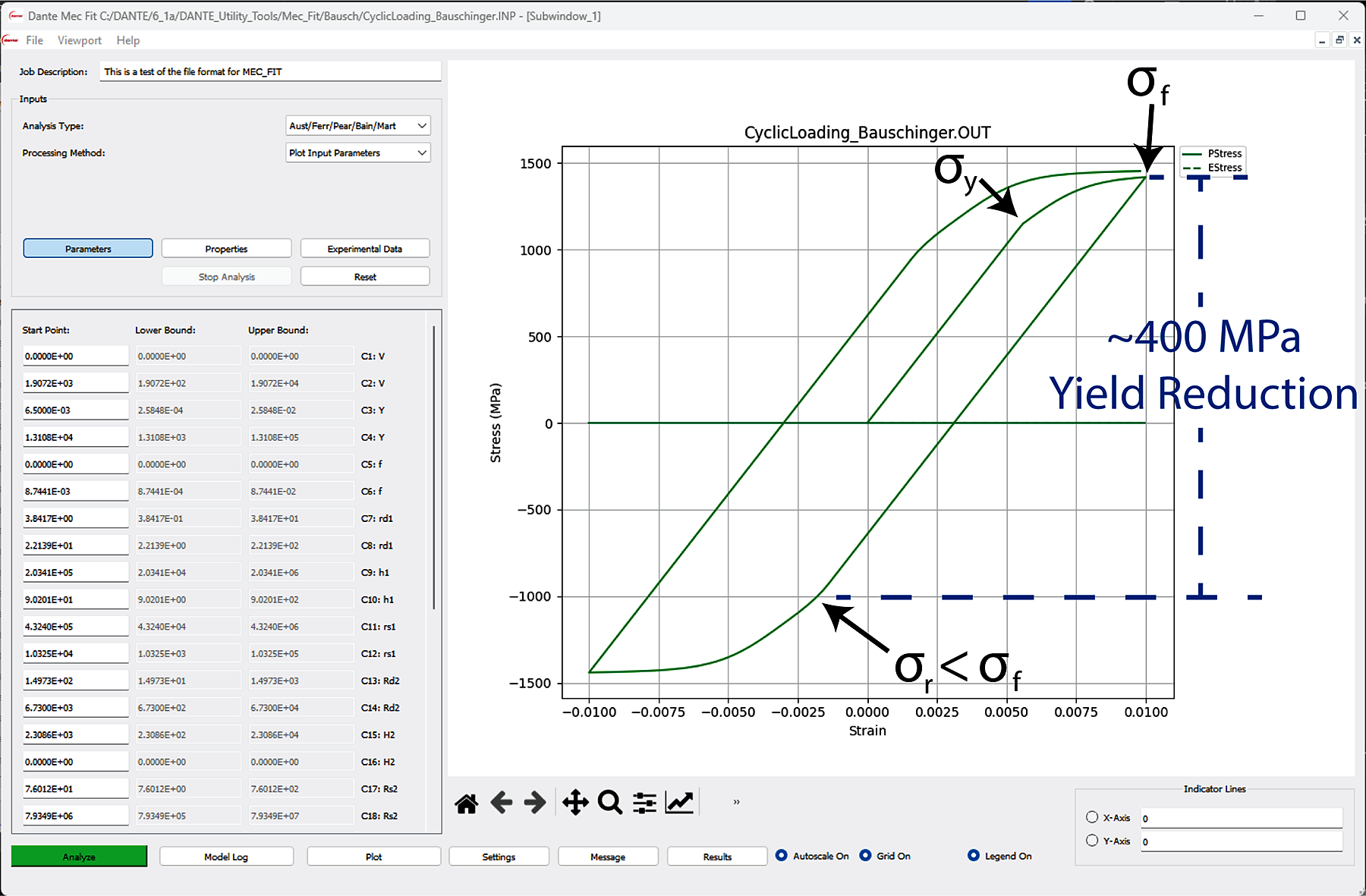
Initially the simulation starts at the origin where a tensile load is applied, after the initial onset of yield, (about 1150 MPa) the material shows some strain-hardening before stopping at 1% strain (about 1400 MPa). The sample is then loaded in compression until it begins to yield at about -1000 MPa, about 400 MPa lower than the strain-hardened sample in tension. Again, we see some strain hardening before the strain is stopped at -1% (-1440 MPa). The sample is finally loaded in tension until 1% strain, where the initial yield is about 1050 MPa. The Bauschinger effect is clearly shown in the difference from the strain-hardened yield and the onset of yield when the load is reversed. Note: there must be some strain hardening to see this effect as the dislocations need to pile up to contribute to the load reversal.
Plastic deformation will always be an important part of the manufacturing process, which can be better understood these days with the use of advanced methods such as FEA. While the Johnson-Cook model is more simplistic than the Baumann-Chiesa-Johnson model, both have been used to describe the general plasticity of metals. The added simplicity and reduced computational costs of the JC model are good reasons for its popularity in FEA. However, the BCJ model offers a more physics-based approach, with its use of internal state variables, allowing it to better capture material behavior such as the Bauschinger effect. It may be a strain to understand these effects, but don’t stress out. Constitutive models can help us to understand and develop new and interesting processes.
References
- Bammann DJ, Chiesa ML, Johnson GC. Modeling large deformation and failure in manufacturing process. Theory of Applied Mechanics 1996; 359–376.


 general practice for CQI-9 and AMS2750E")


